Elementary reaction kinetics
In this section, we shall relate kinetic data to postulated reaction mechanisms
(1) Definition of Elementary reactions
(2) The molecularity of a reaction
(3) Molecularity vs. order
(4) The rate laws of elementary reactions
(5) Consecutive elementary reactions - Variations of
concentrations with time
(5-1) A full inverstigation
of a simple mechanism involving two consecutive recations
(5-2) Approximations
(5-2-1)
The steady state approximation (SSA)
(5-2-2)
The rate-determining step approximation (RDS)
(5-3) More complicated
mechanisms - The concept of a pre-equilibrium
Elementary reaction kinetics
... relating kinetic data to postulated reaction
mechanisms
(1) Definition of Elementary reactions
- Most reactions occur in a sequence of steps called elementary reactions.
- Elementary reactions involve only a small number of molecules or ions.
- The phase of the species in the chemical equation for an elementary reaction is usually not specified.
- The molecularity of an elementary reaction is the number of molecules coming together to react in an elementary reaction. Thus,
- In a unimolecular reaction, a single molecule shakes itself apart or its atoms into a new arrangement, as in the isomerization of cyclopropane to propene.
- In a bimolecular reaction, a pair of molecules collide and exchange energy, atoms, or groups of atoms, or undergo some other kind of change.
It is most important to distinguish molecularity from reaction order:
- The reaction order (first order, etc.) is an empirical quantity, and obtained from the experimental rate law.
- The molecularity (unimolecular/bimolecular) refers to an elementary reaction proposed as an individual step in a mechanism.
Rule: The rate law for elementary reactions may be deduced directly from their molecularity. In fact:
(A) The rate law of a unimolecular elementary reaction is first-order in the reactant:
where P denotes products (several different species may be formed). A unimolecular reaction is first-order because the number of A molecules that decay in a short interval is proportional to the number available to decay. Therefor the rate of decomposition of A is proportional to its molar concentration.
(B) An elementary bimolecular reaction has a second-order rate law:
A bimolecular reaction is second-order because its rate is proportional to the rate at which the reactant species meet, which in turn is proportional to their concentrations. Therefore, if we believe that a reaction is a single-step, bimolecular process, we can write down the rate law (and then go on to test it). Bimolecular elementary reactions are believed to account for many homogeneous reactions.
Note that the converse of this rule does not follow, that is, for example
second-order
rate law does not imply that the reaction is bimolecular - the reaction
might be complex ! Also, care must be taken to ensure that the reaction
/step that we are considering is really elementary. For example, the reaction
H2(g) + I2(l) -> 2HI(g) may look simple, but it is
not elementary, and in fact, it has a very reaction mechanism, and hence
a complex rate law.
(5-1) A full investigation
Some reactions proceed through the formation of an intermediate (I), as in the consecutive unimolecular reactions:
For such a process we have:
(1) The concentration of A is (i) decreasing through unimolecular decomposition of A, and (ii) is not replenished. Thus we have:
.(eqn. 1)
(2) The intermediate I is (i) formed from A at a rate ka[A], and (ii) decreases through decay to P at rate kb[I]. Thus we have:.(eqn. 2)
(3) The product P is (i) formed from I at a rate kb[I], and, (ii) is not decreasing. Thus we have:.(eqn. 3)
Also:
(1) From eqn. 1 we obtain:
Through these equations we may deduce that (see fig. 1):.(eqn. 4)
(2) By substituting eqn. 4 in eqn. 2 and setting [I]0 = 0, we get:.(eqn. 5)
(3) Since at all times, [A] + [I] +[P] = [A]0 , it follows that:.(eqn. 6)
- The concentration of the reactant A decreases exponentially with time;
- The concentration of the intermediate I rises to a maximum and then falls to zero;
- The concentration of the product P rises from zero towards [A] 0.
We may also deduce that the concentration of the intermediate I is at a maximum when:
i.e.:
i.e.:
Consecutive elementary reactions - Variations of Concentration
with time
(5-2) Approximations
It is important to note that there is considerable increase in mathematical complexity as soon as the reaction mechanism more than a couple of steps, and in fact, a reaction scheme which involving many steps is nearly always unsolvable analytically, and hence alternative methods of solution are necessary. One approach to such a problem is to integrate the rate laws numerically. However, other approximation methods are possible.
An alternative and more common to numerical intregration approach is to invoke the so called steady-state approximation.
The steady-state approximation (SSA) assumes that, after an initial induction period (i.e. an interval during which the concentrations of intermediates, I, rise from zero, see fig. 2) the rates of change of concentrations of all reach intermediates are negligibly small, i.e.:
The SSA approximation significantly reduces the complexity. For example, in our case, where the meachinsm is given by:
eqn. 2 would become:
i.e. we may assume that:
and hence:
and so we see that P is formed by a first order decay of A, with rate constant ka (= the rate constant of the slower, rate-determining step). Hence from these deductions and from eqn. 4 we can write down:
as obtained before (though through a much longer process).
The SSA is however not always valid. To be valid, we require a scenario
where the concentrtaion of intermediates must remain small and
hardly change during most of the course of the reaction. In other
words, the concentration of I in the course of the reaction must be described
by Fig. 2 not by Fig. 1.
|
|
|
| Fig. 1 - In this case [I] (blue curve) does not remain small in the course of the reaction. Instead it is constantly changing. this means that the SSA cannot be applied on I. | Fig. 2 - In this case [I] (green curve) remains small in the course of the reaction and hardly changes during most of the course of the reaction (after the equilibration stage). This means that the SSA can be applied on I. |
Mathematically, the required conditions for the SSA to be vaild are that [I] << [A] & [P]. Thus since we have:
then under the SSA we must have:
i.e. we requre that:
In other words, the first reaction producing intermediate I must be slow relative to the rate at which intermediate I reacts and is depleated. This will not allow intermediate I to accumulate as happened in Fig. 1. In fact, the greater the difference between teh two rate constants, the more accurate the SSA will be.
(5-2-2) The rate determining step
Let us once agian consider the mechanism:
Once agian we shall however assume that kb >> ka . In such a scenario, whenever a molecule I is formed, it decays rapidly to P. (Note that these are essentially the same conditions that were required for the SSA, and in fact, we will be getting the same result.)
Mathematically speaking, referring to the full mathematyical derivatiuon in section (5.1) we have:
i.e. eqn. 6 reduces to:
which shows that the formation of the final product P depends on only the smaller of the two rate constants. In other words, the rate of formation of P depends on the rate at which I is formed, not on the rate at which I changes into P. For this reason, the step
'A -> I' is called the rate-determining step of the reaction.
Note: Similar remarks apply to more complicated reaction mechanisms,
and in general the rate-determining step is the one with the smallest rate
constant.
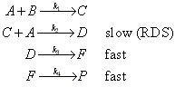
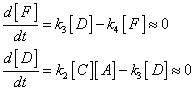
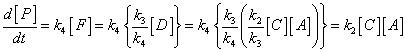
| . | IMPORTANT ASIDE:
The full statement of the rate-determining step approximation states that in a series of consecutive elementary rections the rate of production of the final products depends only the rate coefficient for the last slow step in the sequence and all the rate coefficients preceeding it. For example, consider the reaction: with a mechanism: In this case, compounds C, D and F are intermediates. If k3 and k4 are large relative to k2, than the SSA can be applied to intermediates D and F. This means that after the initial induction period, it can be assumed that: i.e.: and: However, a similar approximation cannot be made for [C] since the SSA does not apply. Thus, since the rate of product formation is given by: then we may write that: i.e.: This shows that the rate of production of P is independent of both k3 and k4 - It only depends on the rate coefficient for the last slow step (i.e. the RDS). Note that beacuse C is also an intermediate, then the rate coefficient of the previous steps and hence in this case k1 will also be implicitly involved. Reference: Lionel M. Raff, Principles of Physical Chemistry, pg. 1128.
|
(5-3) More complicated mechanisms - The concept of pre-equilibria
Let us now focus our attention to a slightly more complicated mechanism in which an intermediate I reaches an equilibrium with the reactants A and B, i.e.:
where the rate constants are ka and k'a for the forward and reverse reactions of the equilibrium and kb for the final step. This scheme involves a pre-equilibrium, in which an intermediate is in equilibrium with the reactants.
A pre-equilibrium arises when the rates of formation of the intermediate and its decay back into reactants are much faster than its rate of formation of the products, that is, when k'a >> kb but not when kb >> k'a. Since we are assuming that A, B and I are in equilibrium we may write:
From now onwards, we may take two approaches:
(1) We assume that the rate of reaction of I to form P is too slow to affect the maintenance of the pre-equilibrium. In such cases we have:
(i.e. the rate law has the form of a second-order rate law).
(2) We assume that reaction of I to form P may affect the maintenance of the pre-equilibrium. In such cases we have:
where through the steady state approximation we obtain:
i.e.:
Note that if ka`>>kb then this last equation will reduce to the one in approach (1).
Note: An application of all this theory may be found in the Michaelis-Menten
mechanism which is discussed at a later stage.