A topological space is a set with a concept of convergence to a point, written \(\color{purple}A \to x\).
A "point" need not mean a literal point but may itself be a set, such as an image.
There is an ideal convergence to a point — its neighborhood (in yellow above) — which selects which other points surround any particular point. Then a set converges to a point if it is eventually inside any neighborhood of it. A converging sequence, \(\color{purple}x_n\to x\), is a special case of shrinking set.
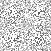
Let's use the set below to illustrate some concepts of topology.
Given the set, one can distinguish three types of points. When you click on any point, its neighborhood is eventually one of three types:
an interior point — the converging neighborhood is eventually completely inside the set;
a boundary point — the converging neighborhood is neither in nor out of the set;
an exterior point — the converging neighborhood is eventually completely outside the set.
A set without its boundary (i.e., just the interior points) is called open; a set with all its boundary is called closed. A set can be closed by adding the boundary.
A set consisting of boundary points only
A dense set has no exterior points.
A set is connected when it cannot be partitioned into two or more parts which are in the exterior of each other.
Sets split up into maximally connected closed pieces, called components. The set above has three components, including an isolated point.
The real numbers are connected; but the natural and rational numbers are totally disconnected.
A set is compact when it is impossible for a set inside it to shrink to nothing.
A compact set must be closed and not extend to "infinity". The set on the right is not compact: it allows subsets to escape to nothing in two ways; the set above, by comparison, is compact.
Any closed subset of a compact set is compact; as is the union of two compact sets.
A discrete space has separated points: a sequence converges when it eventually is constant at its limit. The set of integers \(\mathbb{Z}\) is an example of a discrete space. They are necessarily totally disconnected, and only finite subsets are compact.
Continuity
A continuous function is one which preserves convergence: \(\color{purple}A\to x \Rightarrow f(A) \to f(x)\).
continuous
discontinuous
Click on the graphs
Mapped by a continuous function, a connected set remains connected, and a compact set remains compact.
The squaring map is continuous, so it maps the connected set \([1,2]\) to the connected set \([1,4]\). Since the latter contains the number \(2\), there must be a real number in \([1,2]\) which squares to \(2\); it is called \(\sqrt2\); similarly there is \(\sqrt[5]3\), ...
Products of Spaces
For product of spaces, convergence is determined by the shadows: (click inside)
There are products with any number of spaces, even infinite. The familiar 3-D space can be thought of as a product of three copies of \(\mathbb{R}\), the real line. The product of compact sets is again compact.
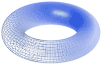
The product of two circles is ... ... a torus.
Types of Topologies
Depending on how the neighborhoods are defined, it may happen that convergence to \(y\) forces convergence to \(x\), when \(x\) is "hidden" underneath \(y\), so to speak; \(y\) is a boundary point of \(x\). One can write this as \(x \prec y\), and an order is determined. Convergence to the deeper "layers" may still be possible using a "finer" neighborhood; but other points may be completely indistinguishable topologically.
For example, convergence of sequences in \(\mathbb{N}\) is usually defined to mean that the sequence is eventually constant, e.g., \(1,4,3,3,3,3,...\to3\) ; but one can define convergence in other ways: let a sequence converge to \(m\) when it is eventually above it, e.g., \(1,3,2,3,4,3,5,3,...\to 3\); but then note that if \(x_n\to3\) then automatically \(x_n\to2,1,0\).
A topology on a finite number of points is necessarily of this type, and is identical to an ordered space. Convergence is thus only interesting and novel when the set is infinite.
\(T_1\) Spaces
A topology is called \(\color{red}T_1\) when there is only one layer of points, with no underlying "hidden" points. Each neighborhood converges to a single point only. Each point is closed and has no other boundary points.
Even so, it may be that other sets converge to several points. In the example to the left, with the neighborhoods defined by yellow sets, the red point (but not the blue point) converges to every point you click on, because it remains in its shrinking neighborhood. The reason is that the neighborhoods all have a common part and fail to dissociate from each other.
\(T_2\) Spaces
A Hausdorff Space is one where a set can converge to only one point; equivalently, any two neighborhoods dissociate from each other as they converge, so that a set shrinking with it has no option but to converge to one point, called its limit.
Any dense subset contains all the information about convergence.
\(T_{3.5}\) Spaces
A Tychonoff Space is even better-behaved: the points between any closed set and any exterior point can be graded continuously, with their neighborhoods following the gradation. In particular a set cannot converge to two points: following a neighborhood, i.e., a color, it can only home in on one of them.
It turns out that every Tychonoff space can be embedded as part of an infinite-dimensional cube. Closing, or completing, it in this cube turns it into a nice compact space.
Every connected subset of a Tychonoff space is uncountable if it has more than one point.
Most practical examples of topological spaces are Tychonoff.
Metric Spaces
A metric space is one where there is a distance between points. Convergence to a point is then determined by a shrinking distance to the point. Requirements for a distance:
any two distances in a "triangle" must add up to more than the third distance;
there are no hidden points, i.e., any two points have some positive distance.
Metric spaces are automatically Tychonoff spaces because the distance can be used to make the gradation between sets.
The real line \(\color{purple}\mathbb{R}\) and its subsets are the classic examples of metric spaces. The distance between points is their numerical difference.
A bounded set is one whose internal distances are all less than a number called its diameter. The natural numbers form the simplest unbounded subset of \(\mathbb{R}\).
Separable metric spaces are those which have a countable subset that can approximate any other point. For example, the real line is separable because every real number can be approximated to arbitrary precision by rational numbers, e.g. \(\pi\approx\frac{22}{7}\approx\frac{355}{113}\approx\cdots,\quad e\approx\frac{19}{7}\approx\frac{193}{71}\approx\cdots\).
A set converges when its diameter diminishes to zero around its limit. But it is possible for the diameter to diminish about a "missing point", e.g., the above numbers \(e\) and \(\pi\) are missing from the rational numbers — they are irrational.
A complete metric space is one which has no missing points. Every metric space can be completed by adding these points. For example, the rational numbers are not complete (they lack the irrationals), but can be completed to the real numbers.
The product of two (or finite number of) complete metric spaces is also complete. So the plane, 3-D space, and other Euclidean spaces \(\mathbb{R}^n\), and their closed subsets, are complete metric spaces.
A compact metric space is characterized by being complete and totally bounded (i.e., a finite number of arbitrarily small bounded sets cover it). The disk with its perimeter is compact; any bounded surface/shape in Euclidean space with its boundary is compact.
A function on a complete metric space, which decreases distances between points by a fraction, will converge to a fixed point if mapped repeatedly to any starting point, \[\color{#900}x,\quad f(x),\quad f(f(x)),\quad \ldots\quad \to\quad a,\qquad\qquad f(a)=a.\]
Below, the function \(f(x)=1/(1+x)\) converges to the 'golden ratio' \(0.618\ldots\) which satisfies \(\frac{1}{1.618\ldots}=0.618\ldots\).
Measures and Dimension
Some sets can be given a kind of distance: a size or measure \(\mu(A)\).
The basic requirements are:
the empty set has zero size,
two disjoint sets add up in size,
if \(A \to x\) then \(\mu(A) \to 0\).
Cardinality, lengths, areas, and volumes are the classical examples of measures in Euclidean spaces.
There are fractional measures in between these. A set has zero fractional measure until a particular value of the fraction: this value is called its fractional dimension.
Points have dimension \(0\); lines have dimension \(1\); surfaces have dimension \(2\);etc. The Cantor set has dimension \(\log_3 2=0.63\ldots\)
The Sierpinski triangle has dimension \(\log_2 3 = 1.58\ldots\)
Not every set can be given such a measure or dimension; and several sets, called null, have zero measure, so this is not exactly a distance on sets.
Curiously, any non-empty bounded open set in 3-D space can be broken up and reassembled into any other such set! But the pieces have no assigned size.
Local properties
A property of a topological space may hold in a neighborhood, or it may hold at large. A space may be nice locally, but be very complicated globally; or vice-versa.
The set on the left is connected but not locally connected: any tiny neighborhood of a point on the right-most line consists of disconnected pieces.
Locally compact Hausdorff spaces are special types of Tychonoff spaces: they need only one extra point, called infinity, to become compact. For example, the real line becomes the circle when infinity is added to it...
... and the plane becomes the sphere with the point at infinity being the "north pole". (Click inside to start)
Embeddings
Two topological spaces are essentially the same when they can be transformed into each other continuously, back and forth.
It is impossible to classify all topological spaces. But one can see in what ways a simple topological space can be placed without intersecting itself, or embedded, inside another one.
The circle can be embedded in the plane and in 4-D space in only one (finite) way up to a deformation. But there are many embeddings of the circle in 3-D space, called knots. Every knot can be built up by joining some irreducible ones, the first few of which are (not including their mirror-images):
The number of different knots grows exponentially with the number of crossings.
Similarly, one can classify how the sphere embeds in 4-D space, etc.
Homology
For topological spaces that can be triangulated, one can extract homology groups that contain much of the global information of the space. They consist of closed cycles of points, edges, faces, ... , which are not boundaries of edges, faces, volumes, ... The dimensions of these groups are called the Betti numbers of the space, \(B_n\), e.g., \(B_0\), being the number of non-equivalent ways of placing a point, is the number of connected components, \(B_1\) counts the number of "tunnels", \(B_2\) the number of "voids" , ...; they can be combined to give the Euler characteristic, and used to distinguish topological spaces: \[\color{purple}\text{Euler characteristic } \chi = B_0-B_1+B_2-B_3+\cdots\]
The sphere has one component, no tunnels, and one void (inside), so the Betti numbers are \(1,0,1\); and the Euler characteristic is \(1-0+1=2\).
The torus has one component, two tunnels (corresponding to the two ways of inserting a loop which is not the perimeter of a disk), and one void. The Betti numbers are \(1,2,1\), and the Euler characteristic \(1-2+1=0\).
The Euler characteristic of the disjoint union of two spaces adds up; and of a product multiplies out:
In fact, since the Betti numbers of the circle are \(1,1\), and its Euler characteristic is \(1-1=0\), then \(\chi(\text{torus}) = \chi(\text{circle}) \cdot \chi(\text{circle}) = 0\)