This page contains an applet that demonstrates the use of a general engine that can be used for fast generation of Dynamic Programming (DP) applications. The engine performs the backward procedure of DP with discrete states and discrete decisions when all is deterministic (if this sounds alien to you, no problem, just use the applet).
There is a certain number of planning periods (typically years, months or weeks) for which we know the demand for a certain inventory item. Initial inventory available is known. For each period we know the fixed setup cost paid once. It is either the production setup cost or the fixed order cost. Then we know the unit cost per item produced or ordered. Holding is the cost paid per item held in inventory at the end of the period. Stockouts are allowed, but they are resolved at the end of the period for extra setup cost per unit. So each period starts with a nonnegative inventory. All these figures are generally different in each period. We want to find the production/order at all periods that would minimize the total cost while keeping all restrictions satisfied. To speed up the solver, it is very important to enter the maximum possible inventory and the maximum possible production or order. Minimum inventory can also be given. If stockouts are allowed, the minimum inventory must be negative. After the last period we assume zero inventory level. If this is not the case, the closing inventory has to be included in the last demand. Note that the actual cost of the items involved is not included in the model, but interest lost by keeping the inventory is typically included in the holding cost.
First of all your browser must be able to run Java applets. If the box underneath is filled in, it is. There are two text areas. The first contains the problem data in table form, the second contains the results. Note that there is a default instance of the problem. Press the button Solve and you are supposed to obtain the result similar to the following one:
 DP Solver v4 start: Thu Jun 14 15:13:17 CEST 2007
 Total time taken  : 0 ms

 Number of stages  : 5
 Initial status    : 0
 Optimal objective : 2070.0
 Optimal plans     : 1

 44 65 0 76 0
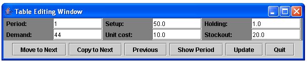
Compare the optimal plan with the demand and note that due to setup costs in two periods it is cheaper to produce for two periods even if extra holding cost is paid. The button Generate Default Data copies the entered costs into all periods, the demand is generated randomly in the given range with equal probabilities. Press the button Edit to start the editing session in a window similar to the following one:
Use the buttons Move to Next and Previous to display data from the next/previous table entry. The button Copy to Next copies data from the current to the next table entry. Enter the period number and press the button Show Period to move fast in the table. Press Update to change the table entry according to the data entered in the text fields. All changes are shown in the data text area, all validation is performed and reported in self-explaining way.
You may skip this section if you are not interested in DP and Java. The engine contains the general algorithm common to all applications. It solves the optimization problem by the backward procedure and retrieves all optimal plans. The results are supplied by the result object that contains the status of the first stage, the optimal objective value, and all optimal plans in a 2-dimensional array. Features given by the particular application, here the inventory problem, are included as methods of the class Application. The engine requires methods that return the following:
Set of states for a given stage
Set of decisions for a given stage-state pair
Transition - the status of the next stage for a given stage-state pair and a given decision
The return value for a given stage-state pair and a given decision
The result of combining a given return and an optimal objective of the next stage (here and in most cases just their sum)
The objective associated with the transition generated by the last stage that is needed to solve the last stage. For the inventory problem this value is 0.
Compared with the engine the methods are very simple. As an example, here is the method that computes the return where t is the stage number, yt is the status (inventory level from the previous period) and xt is the decision (number of items produced/ordered at this period).
  // freturn(t,yt,xt) returns the cost (return) of decision xt at (t,yt)
  public static double freturn(int t,int yt,int xt) {
    double rt;
    if (xt == 0)
      rt = 0.0;
    else
      rt = setup[t] + xt*unitcost[t];      // production/order cost
    int atend = yt + xt - demand[t];       // closing inventory
    if (atend > 0)
      rt = rt + holding[t]*atend;          // add holding cost
    else if (atend < 0)
      rt = rt - stockout[t]*atend;         // add stockout cost
    return rt;
  }
Data that define the particular instance of the problem are stored in variables of the class Application. The solver writes these data before calling the engine. The following is the method called after pressing the button Solve where result is the text area in the applet window and solverResult is the object to store the result (common to all applications). Names of variables are self-explaining.
  void callSolver() { // Prepare data and call solver
    Application.T = T;
    Application.demand = demand;
    Application.initial = initial;
    Application.setup = setup;
    Application.unitcost = unitCost;
    Application.holding = holding;
    Application.stockout = stockout;
    Application.mininventory = minInventory;
    Application.maxinventory = maxInventory;
    Application.maxprod = maxProd;

    DPEngine4 engine = new DPEngine4();
    solverResult = engine.solve();

    result.setText(solverResult.toString());
  }
An engine version in Matlab is also available. The purpose of the engine is to support fast, relatively easy implementation of DP solutions manageable by students who are not experienced programmers.