PetriSim 5 Manual

PetriSim is a generator of discrete simulation models that can also be used as a graphical editor and simulator of Petri networks (P-nets). Two languages are used to create simulation models. First the P-nets graphical language defines the basic structure and relationships in the model. Details that cannot be incorporated in the network model are then expressed by Pascal (the host language of PetriSim is Turbo/Borland Pascal 7). User Pascal code is made of a number of very short snippets, because most statements just call methods of classes supplied in supporting units. From version 5 of PetriSim user programming is limited to special cases, for example the situations when firing duration depends on marking of some places. Most models will be created by editing the network that includes entering of all parameters of places and transitions without writing any code snippets. PetriSim is an educational tool that can be used in all courses that teach:

· Discrete Simulation

· Petri nets and their modifications

· Object Oriented Programming.

The problem addressed by PetriSim is this: creating discrete simulation models in general high level languages is very difficult, learning simulation languages (like for example Simscript) takes time. Today there are of course powerful (mostly expensive) visual simulation tools like for example Extendä or Arena^TM. PetriSim is a free easy to use tool. The most difficult part of discrete simulation - model timing and synchronization - is done by the graphical language of P-nets. The rest is Pascal programming that most students already know. All that students have to learn are basic ideas of P-nets. Unlike other P-nets based tools, PetriSim nets are very close to the basic Place/Transition (Pl/Tr) nets - in fact the only extension is firing duration that incorporates time, generalization of arcs and branching transition – see later. So we call the nets Time nets (T-nets). Firing duration together with P-net topology create complex timing and synchronizing structures, that are normally programmed by special statements of simulation languages. There are no complicated definitions used in most theoretical high-level Petri nets. Additional functionality, if needed, is added by user code associated with transitions. PetriSim uses P-net as a descriptive tool only. There is no attempt to use analytical capabilities of P-nets.

PetriSim enables a very user-friendly creation, editing, and simulation of practically any number of P-nets at a time. Most operations are performed by drawing by the mouse on the screen. Networks can be stored in disk, they can be updated and renamed, so it is possible to work simultaneously on several versions of one network model. Work is made easy by on-line context sensitive help.

The fact that user programming will not be used in most models is not paid by limited generality and flexibility of PetriSim based models. Functionality and flexibility achieved by user programming is not limited, all standard procedures can be replaced by user-defined ones.

2. PetriSim Networks

2.1 Place/Transition Networks

Definition: The Marked Petri Net (P-net) called also Place/Transition or Pl/Tr net is a 5-tuple (P,T,I,O,M) where P and T are non empty finite sets of places and transitions respectively. P Ç T = Æ .

I is the so called Input function: I: PxT ® N , where N is the set of non negative integer numbers. The value I(p,t) is the number of (directed) arcs from the place p to the transition t. There can obviously be no arcs if I(p,t) = 0.

O is the so called Output function: O: TxP ® N , where the value O(t,p) is the number of arcs (possibly none) from the transition t to the place p.

So the 4-tuple (P,T,I,O) is a bipartite directed multigraph whose arcs connect vertices from 2 distinct sets (P and T).

M is the initial marking of places: M: P ® N , where the value M(p) is the number of the so called tokens that are located in the place p.

Interpretation: A transition is enabled if all places contain at least so many tokens as is the number of arcs from the place to the transition. A transition that is not enabled is disabled. An enabled transition may be fired. During firing every arc whose endpoint is the transition removes one token from its starting (input) place and every arc starting at the transition adds one token to its ending (output) place.

From modeling point of view places represent certain conditions that must be true for some activities (transition firing) to start. Firing changes the marking of both input and output places. This may enable or disable other transitions, etc. All enabled transitions that are not mutually exclusive may be fired in parallel.

Drawing:

Places are drawn as circles that are either empty or that contain some number of tokens. Because of practical reasons PetriSim does not draw tokens as small filled circles but every place contains a non-negative integer number of tokens. Name of the place is displayed at the bottom right of the place.

Transitions are drawn as short thick lines. PetriSim also displays the name at the bottom of the transition. PetriSim allows either horizontal or vertical (default) direction of a transition. Enabled transitions are displayed with a mark:

Arcs are lines finished by an arrow. Points where arcs start/end are defined by the user. PetriSim allows any length and shape of arcs.

Note: Starting from PetriSim version 3.1 there are various place and transition icons to improve readability of networks. It is also possible to create inhibitor arcs that end by a small circle and test arcs that are just lines.

Application:

Petri nets offer a very natural and lucid way of expressing co-operation and communication of parallel processes. This is very useful when modeling computer and communication systems but there are many other application areas. There are many extensions to the basic Pl/Tr nets improving the modeling power. These extensions are called High Level Petri Nets. Petri nets have also powerful analytical capabilities not used by PetriSim.

2.2 Time Networks

The so-called Time networks (T-nets) introduce time. There are several approaches how to cope with time in Petri and related networks. PetriSim is based on the "firing delay" approach. It means that firing takes a certain time. When applying the firing delay way of introducing time to P-nets, three problems have to be resolved: firing semantics, conflict resolution policy, and nature of firing delay. In PetriSim these problems are solved as follows:

Firing semantics defines three stages. When a firing starts, the tokens are removed from input places of the transition (this represents the fact that a certain activity has started). During firing the tokens are "hidden" in the transition. When the firing ends, the tokens are added to output places of the transition (a certain activity has terminated). Analytical properties of this abstraction are irrelevant, because PetriSim uses T-nets as a descriptive tool only.

Conflict resolution policy is in PetriSim 5 based on priorities of transitions. Priority is an integer value in [0, 65535], the default value is 100, 0 is the highest priority. If there are more enabled transitions with the same highest priority, the one to be fired is selected randomly, all with the same probability. In some step simulation modes the transition to be fired is selected by the user.

Nature of firing delay is not restricted. All transitions are by default immediate ones with constant firing delay 0. The user can select other constant delay or a random delay. Several theoretical distributions are available, see later, alternatively it is possible to enter an empirical table. Starting code snippets written by the user can override the entered delay by computing any deterministic or random delay, for example such that depends on the network status (marking of some places).

Graphically T-nets look like P-nets, the only difference is visible during a user experiment in debugging mode when transitions in "firing on" status are displayed in different way together with the firing completion time. The same graphical editor is used to create and edit both types of nets. So from now on the abbreviation "P-net" represents both types of networks. P-net is in fact a special case of the T-net with zero firing delay of all transitions.

Firing delay and time as such exist only in the so-called user mode - see the description of the menu option Simulation in the chapter 4.4. Each PetriSim net can thus be simulated as a P-net (no time) or as a T-net with delays. Delays are either entered by the user during network creation or editing, or generated by starting code snippets. Every transition can have a starting code snippet (activated when firing starts after removing tokens) and an ending code snippet (activated when firing ends before adding tokens). These code snippets are written by the user when editing the network in PetriSim (not off-line in Pascal IDE). From Pascal’s point of view the snippets are separate .PAS files, so they can be later edited (mostly corrected) in Pascal IDE.

3. Simulation in PetriSim

The following main steps are involved in building simulation models in PetriSim environment:

· Informal description of the system simulated

· Creating a P-net model

Experimentation with the P-net model

· Creating a user model on the P-net skeleton

· Experimentation with the user model.

PetriSim supports the last four steps.

a) Informal description of the system simulated is the first step of all simulation studies. When using PetriSim it should be made in such a way that supports identification of parallel processes and their interaction. Instead of parallel processes it is also possible to state clearly necessary conditions and results of all activities. Of course these two approaches may be combined.

b) Creating a P-net model starts by expressing the conditions in P-net terms. There is no general guide how to do this. The only way is studying other network models because the number of typical constructs is not big. The P-net can be built in incremental way by repeated additions to simpler nets. PetriSim supports this approach. It is always possible to add any number of new places and new transitions and to create new arcs between them. Arcs can be deleted; places and transitions can be made invisible. The P-net can always be stored in a disk. Because the user can define the file name, it is possible to keep more versions of the same network model. PetriSim package includes some demonstration examples explaining basic ideas and typical P-net constructs.

c) Experimentation with the P-net model is supported by several simulation modes that do not work with time. These modes differ in the degree of user control over firing of transitions. If there are more enabled transitions with the same priority, the user can either select the transition to be fired or the selection can be done randomly by PetriSim (equal probabilities). Some modes are based on user action before firing a transition. These step modes enable detailed studying and analysis of network behavior. There are also two automatic modes with and without delay between firing. The fast mode is supposed to be used when searching for deadlocks. P-net simulation checks basic logical relationships in the model, especially all kinds of communication and co-operation procedures and mechanisms. All cases when the network behavior depends on firing duration must be in these modes simulated by careful user’s selection of the transition to be fired.

d) Creating a user model on the P-net skeleton is necessary in order to generate firing delays and/or to obtain non-standard results. In PetriSim 5, most models are created by entering firing delays and probabilities of branching transitions – see later. User code that is needed only in special situations is made of the Pascal unit USER and various code snippets, that are in fact include files inserted at compile time. Include files and include directives are generated by PetriSim, the user writes only the code. From Pascal's point of view a snippet is a procedure without parameters whose heading is generated by PetriSim. Generic version of the unit USER is provided. USER units of various models will be very similar - in fact there is no need to change anything if you have no additional user data and if you are satisfied with standard outputs. Model-specific features include:

Declaration of model specific variables (modified during the experiment by code snippets)
Initialization of the model
Experiment evaluation

Complexity of user code is practically not limited. A user can declare any number of procedures and other objects to be used for animation, presentation graphics, etc. Chapter 5 deals with user models in more detail.

e) Experimentation with the user model is also supported by PetriSim. Simulation setup includes the possibility to work in step mode. It means that the user can display the network at each event. All transitions in "firing on" status are marked together with firing completion time. This supports a detailed analysis of network behavior. For details see the chapter 5. Other setup options include the duration of the experiment and the output format, whether the results on places and transitions are generated separately or in two concise tables.

4. Work with PetriSim

PetriSim supports interactive creation, modification, and simulation of P-nets. PetriSim networks are class instances, so the user can create and keep in memory (or in disk) any number of network models. Free RAM capacity (even in real mode) enables keeping tens of P-nets in RAM at a time. There is also some room to load COMMAND.COM (DOS Shell) and the text editor. PetriSim works practically on any IBM PC compatible computer. PetriSim is an MS DOS application that can be started in Windows 3.x, Windows 95/98/Me/XP and NT platforms (so far we haven’t found any incompatibilities).

The program PETRISIM.EXE can be placed anywhere, but the suggested way is this: create the directory C:\PETRISIM and for each model its own subdirectory - e.g. C:\PETRISIM\PACKETS. In each subdirectory there are files related to the particular user model. There is the program PETRISIM.EXE compiled for this user model, and also a simple menu program PSIMMENU.EXE that starts typical activities involved in model building (PetriSim, Pascal, Text Editor, File manager, DOS Shell). To start work with PetriSim start the short batch file S.BAT that activates PSIMMENU.EXE, e.g.:

C:\PETRISIM\PACKETS>S

In Windows platforms it is suggested to create a folder called PetriSim with separate shortcuts for each model. In fact all model shortcuts will start the S.BAT file in various working (model) directories like C:\PETRISIM\PACKETS. It is also possible to start PETRISIM.EXE directly, especially if you do not have Pascal. Note that without Turbo or Borland Pascal IDE you are limited in the generality of user models, but starting from version 5, most models do not need any user programming. PetriSim can be used also as an editor and simulator of Petri-based networks without time but with generalized inhibitor and testing arcs. Alternatively it is possible to do all the work from the Pascal IDE, especially during creation and debugging of the user model. To start PetriSim run PETRISIM.PAS from Pascal (Ctrl-F9). After creating or editing a code snippet (see later), return back to Pascal IDE and run PETRISIM.PAS again – this will re-compile it. The following picture is the main menu of the PetriSim environment displayed by PSIMMENU.EXE:

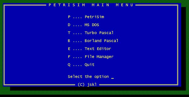
Figure 1: The main menu of the PetriSim environment

The above menu options are self-explaining. Modify and recompile the program PSIMMENU.PAS to adjust it to your computer and taste. The supplied version assumes standard installation of Turbo/Borland Pascal in C:\TP and C:\BP respectively. The MS DOS shell is C:\WINDOWS\SYSTEM32\COMMAND.COM, the text editor is C:\WINDOWS\SYSTEM32\EDIT.COM. The file manager DOS Controller^TM (freeware - Author: Søren Kragh, 1992) is included in model directories (files DC.*). Note that the main menu is very simple because in real mode there might be problems with memory. Change the memory directive {$M 16384,0,250000} in the 3rd line of the program PETRISIM.PAS to adjust the heap and the area left for utility programs, that is used for the text editor when creating/editing code snippets. Avoid any memory problems by selecting the protected mode (Borland Pascal only).

4.1 Menu

PetriSim menus have the usual tree structure. The options of the main bar menu (except Quit) activate pull-down submenus; some options of them activate other submenus, etc. Some options open dialogue windows used to enter names and numerical parameters. There are unified rules how to activate menu options:

By mouse: select the option by the mouse pointer and press the left mouse button. The selected option appears in a rectangle - see Figure 2. If an option has no highlighted character, it cannot be activated. Close the menu by the right mouse button.

By keyboard: either press the hot key of the option (the highlighted character) or select the option by arrow keys and press Enter. The selected option appears in a rectangle. If an option has no highlighted character, it cannot be activated. Close the menu by the key Esc. If you have an open submenu at the first level, it is possible to move among pull-down menus by horizontal arrows. So use vertical arrows to select the menu option.

Activating menu options by the mouse and by the keyboard may be freely combined (selecting by mouse and pressing Enter, selecting by arrow keys and pressing the left mouse button, etc.) Letter keys are of course not case sensitive.

Closing the main bar menu (by the right mouse button or Esc) ends the PetriSim session (like Quit). If there are any networks in RAM, the exit must be confirmed by the key Y (not by mouse) because it is possible to loose a lot of work on networks not saved in disk.

4.2 Creating networks

To create a new P-net use the option Create of the submenu activated by the option File of the main bar menu. (Notation File - Create will be used from now onwards.) The screen in Figure 2 has been captured immediately before activating this menu:

Figure 2: Activating the menu option File - Create

After activating File – Create PetriSim opens a window to enter a name of the new P-net. The maximum length of the name is 8 characters and only those characters allowed in MS DOS file names will be accepted. It is because the P-net name becomes the default name of the file to which the P-net will be saved by the option File - Save (see later). It is not possible to enter the name of a network that already exists in RAM (names of P-nets are not case sensitive).

Initially the P-net exists as an instance of the class describing P-nets as such. All parameters have default values; lists of places and transitions are empty. So the screen is empty because the new P-net has been automatically selected as the active one. Check this by the option Management - List of nets that displays a list of all networks in RAM in the order of their creation or loading from disk respectively. The selected (active) P-net is displayed in highlighted color. To select other P-net use the option Management - Select. To resolve any clashes of network names use the option Management - Rename. To change the name the network need not be selected. The rules mentioned above hold also for entering the new name that of course must be unique.

After creating an empty P-net, the typical next activity is its interactive building by creating its places and transitions and by connecting them using input and output arcs. This is explained in the next chapter.

4.3 Editing networks

To edit a network, it must be selected (if not use the option Management - Select). The selected network is always displayed on the screen with its name in the upper right corner. The option Edit of the main bar menu opens a submenu with three options: Screen editing, Relocations, and Displays. The last two options are intended as a support when working with large networks. Almost everything is normally done in the screen-editing mode (see later) started by the first option.

The option Displays can be used to display the list of all places, the list of all transitions, and the connection of a transition (the list of the input places and the list of the output places of a transition). The screen of a PC is relatively very small. That's why PetriSim allows the user to display only certain parts of a large network. Any arc can be left invisible, but it exists and it is taken into account during simulation. Similarly it is possible to hide a place or a transition by moving them to the left side of the screen (x co-ordinate = 0). The lists mentioned above contain all objects - both the visible and the hidden ones. So use this option in case of any uncertainty.

The option Relocations can be used to display again a hidden object (a place or a transition). It is because these objects are not visible and so they cannot be moved by the mouse. This option at first opens a window to enter the name of the object being relocated. Note that names of places and transitions are case sensitive! Use the option Edit - Displays to get the exact name of the place or the transition. After entering the name, click the left mouse button at the new location of the center of the relocated object. It is possible to relocate any object (not only a hidden one), but objects not hidden can be very easily moved by mouse without entering the name.

To display again an invisible arc, create it once more. When creating an arc, the previous one connecting the same two objects in the same order is deleted (if it exists).

The option Screen editing starts the screen-editing mode. This mode has its own main bar menu (to keep the screen as free as possible) that allows the user to create new objects (places, transitions, and arcs), to activate certain global operations on the net as such, to display the context Help (F1), and to finish the screen editing mode (Esc). Other editing operations are performed directly by the mouse. (Using keyboard is also possible, but not recommended. In this case the mouse driver must not be installed!) The Help displays the rules explained in this chapter. The right mouse button is used for editing operations. So it is not possible to use the right button to finish the screen-editing mode (use Esc, or the associated menu option). Without mouse the right button is simulated by Esc (the left one by Enter). To finish screen editing without mouse use F10.

During most editing operations there is a prompt at the bottom of the screen stating exactly what is going on.

4.3.1 Creating Places and Transitions

To create new places and new transitions use the options New: place or New: transition respectively. After pressing the left mouse button the new object appears at the top of the screen. The new objects have the current default parameters (size and color). New places are given default names p1, p2, ... etc. A new place has the marking equal to 0. New transitions are given default names t1, t2, ... etc. A new transition has the vertical direction. All these can be easily changed.

To move a place or a transition select it by the mouse pointer and drag it (by the left button pressed) to the new location. The movement stops by releasing the left button. With places and transitions also the ends of incident arcs are moved. Moving arcs means moving just the endpoints of the first or the last segments (the relative replacement of the endpoint is equal to the relative replacement of the place or the transition). Other segments of the arc can be easily relocated later. Places and transitions moved to the leftmost side of the screen become hidden (not displayed). Hidden objects are of course taken into account during P-net simulation. Use the option Edit - Displays to get the list of all objects - the hidden objects have the x co-ordinates equal to 0. Use the option Edit - Relocations to place a hidden object back to screen.

4.3.2 Creating Arcs

To create a new arc use the option New: arc. The option then prompts for the starting place (input arc) or the starting transition (output arc). Then select the ending transition (input arc) or the ending place (output arc). The arc type is given by the first selection. Select the place or the transition by the left mouse button. Then it is possible to leave the arc invisible (right button) or to draw it (left button). The last option starts the drawing mode. The first and all the other corners (except the last one) are fixed by the left button. Fix the last corner by the right button. A normal arc ends by an arrow, whose orientation is given by the last segment. So it is recommended to end the arc by at least a short straight line. When drawing, the active segment moves with the mouse pointer. This segment can be adjusted to the vertical/horizontal direction by pressing the key V/H. The arc can be later easily modified including inserting and removing corners. By holding the left button pressed, it is possible to draw arcs of any shape. Do not hold the left button pressed too long (especially with fast computers) because the corners are permanently scanned and placed to memory - every corner is a class instance. On the other hand slow computers need slow movement of the mouse - try. Without further editing there is just one arc between two connected objects. For more arcs change the weight of the arc. On the screen there will always be only one line, weight (multiplicity) greater than 1 will be displayed as a number in the first line segment. Note that inhibitor arcs end by a small circle; testing arcs are plain lines.

4.3.3 Editing Place Properties

To edit a place select it by mouse and press the right button. This opens a menu close to the place - the exact location depends on the location of the place on the screen. Figure 3 shows the screen just before editing the name of the place p1.

Figure 3: Editing place properties

There are these menu options:

Change marking - to change the marking of the place (the number of tokens). Note that marking is a non-negative long integer number with the maximum value 2,147,483,647.

Change name - to enter a new name of the place.

Change size - to resize the place by entering a new radius of the circle. If the shape is not a circle - see place type - the size is half the side of an imaginary square around the place icon.

Change color - to change the color of the circle and the color of the name (these colors are equal).

Marking color - to change the color of the marking (the number in the circle).

Place type - to change the type of the place. So far the type affects only the place icon. Various new environments built on the basic PetriSim classes are supposed to use place types. So far it has been implemented in Queuing Nets that use these types:

Circle (default)
Horizontal left to right queue
Vertical top down queue.

For more details see the chapter 6.

Timing is ON/OFF is a toggle that turns on and off collection of statistics on time spent by tokens in the place. Typically it is used for places that model queues of queueing systems. The results then represent the statistics on the waiting time in a queue. With respect to the time spent a place behaves like an FCFS (First Come First Served) queue. Collection of the time spent is implemented by keeping a list of records with arrival times for each token. This may result (especially in real mode) in run out of memory for places where large amounts of tokens accumulate. So it might be a good idea to start experimentation with this option turned off. Simulation will also be faster, but the difference is not significant, unless large numbers of tokens accumulate in some places. The suggested rule might be to turn this option on only for selected places where time spent by tokens in a place is meaningfull. Definitely do not turn this option on for places used as counters. Note that this option has to be turned off if the user snippets change the marking of some places by the procedure ChangeMarking – see later. In this case the lists would not be consistent with the actual number of tokens. The default initial value is OFF.

Most menu options open a window to enter or select the new value. The colors are chosen from another menu in usual way - either by the mouse or by pressing the hot key (hexadecimal color number). When entering the new value use the key Backspace to correct possible typing mistakes. An error in the number is announced by the message together with the position of the error. Try again to enter a correct value. Before entering the new value it is possible to abandon the operation by pressing Enter, Esc, or any mouse button. The original value will not be changed. If the entering has already been started (by pressing a key) it is possible to abandon by Esc, the original value will not be changed. All changes of place parameters are immediately updated on the screen.

Names of places and transitions are made of 1 through 15 characters (all characters including spaces are allowed). The names are case sensitive! It is not possible to enter a name of a place that already exists.

4.3.4 Editing Transition Properties

To edit a transition, select it by mouse and press the right button. This opens a menu close to the transition - the exact location depends on the location of the transition on the screen. Figure 4 shows the screen just before activating the text editor to modify the starting snippet of the transition t1.

Figure 4: Editing transition properties

There are these menu options:

Change direction - to change the direction of the transition - horizontal or vertical (default).

Change name - to enter a new name of the transition.

Change size - to resize the transition (by entering a new length of the thick line). If the shape is not a thick line - see transition type - the size is the side of an imaginary square around the transition icon.

Change color - to change the color of the line and the color of the name (these colors are equal).

Transition type - to change the type of the transition. Various new environments built on the basic PetriSim classes are supposed to use transition types. So far it has been implemented in Queuing Nets that use these types:

Thick line (default)
Timed transition - rectangle
Generator icon - always horizontal
Branching - triangle.

Transitions with different types are shown by different icons, branching transitions have different behavior – see later. See also chapter 6 for more details.

Priority - to change the priority of the transition. Priority is an integer value in [0, 65535], the default value is 100, 0 is the highest priority. Priority is used to resolve conflicts during simulation. If there are more enabled transitions with the same highest priority, the one to be fired is selected randomly, all with the same probability. In some step simulation modes the transition to be fired is selected by the user.

Firing delay - to enter the firing delay of the transition. It is possible to change the default delay 0 to other constant or random value. Random delays can be drawn from theoretical distributions or from empirical tables. Delays entered during P-net editing can be overridden by delays generated by starting snippets. If there is no starting snippet or the starting snippet does not generate a delay, the entered one will be used. By using delays generated by starting snippets it is possible to model for example state-dependent service duration, etc. If an empirical table delay has already been entered, attempt to enter a delay has to be confirmed in order not to overwrite accidentally a possibly long table. The following delays can be entered:

Constant – enter the constant firing duration.

Table discrete – user is prompted to enter a list of possible values together with their probabilities. After entering a probability, the CDF is computed and displayed. Follow usual rules. The sequence of values must be nondecreasing, probabilities must be in [0, 1], their sum should be 1. If not, the CDF is truncated to 1, last CDF is set to 1. In both cases a warning is displayed. Only entered values will be generated.

Table continuous – same rules apply for entering the table. Generated values are computed by linear interpolation. Example: there are values 2 and 5 with CDF's 0.3 and 0.6 respectively. If the internal uniform generator returns 0.5, the generated delay will be 4. A continuous table is supposed to be used as a piece-wise linear interpolation of a continuous CDF.

Exponential – enter the mean value.

Erlang – enter the mean value and the integer shape parameter. The mean value applies to the Erlang distribution, not to the underlying exponential distributions.

Uniform – enter the minimum (m) and the maximum (M) values. m £ M.

Triangular – enter the minimum (m), the most likely (L), and the maximum (M) values. m £ L £ M.

Normal – enter the mean value (m) and the standard deviation (s). Normal values are generated by rormalizing the sum S of 12 random values from (0, 1) as follows: X = m + (S-6)*s.

Normal in n sigma – enter the mean value (m), the standard deviation (s), and the integer number n. The generated values are originally normal, but only those in m ± ns will be returned.

Show & seed menu option displays the current distribution and its parameters. Then it is possible to enter a seed. The standard Turbo/Borland Pascal random generator is used, but every transition has its own seed that is used to generate random delays. So every transition has its own independent stream of random numbers in (0, 1) used to generate random delays. The default seed 0 is not used, the seed is generated before each simulation run by the standard Pascal procedure Randomize. In order to repeat simulation runs with the same sequences of random numbers, enter any integer seed other than 0.

Branching - to enter probabilities of branching transitions that are the only transition type with modified behavior. The token(s) are added to one output place only. By default the output arc/place is chosen randomly, all with the same probability. After activating this menu option the user is prompted to enter probabilities for output places one at a time in the order of creating the output arcs. Usual tests are performed, internally the cumulative distribution function (CDF) is stored. If the sum of probabilities is not 1, user is warned about the fact. All CDF values greater than 1 are truncated to 1, the last value is always set to 1. There is an integer property Branch whose initial value is zero. User code activated at the end of firing can change the value of this property to implement any kind of deterministic or not supported random branching. Value set by an ending snippet overrides the probabilities entered by the user. It is supposed that using ending snippets to generate random branching will be an exception, for example to implement a state-dependent branching.

Starting snippet - to create or edit the starting snippet of the transition that is activated at firing start time after removing tokens from input places. If the starting snippet so far does not exist, PetriSim informs the user by opening a window. User can either cancel the operation (which is strongly suggested, if you are not sure) or create an empty snippet that is similar to this one:

Procedure _PS1; {Starting snippet of the transition t1 (Line1)}
Begin
End;

PetriSim then activates the text editor that displays the code snippet file. Details depend on the editor used. The editor to be used by PetriSim is defined by the string constant EditorName in the Interface part of the unit USERPART. This is the default declaration:

Const EditorName = '\WINDOWS\SYSTEM32\EDIT.COM';

PetriSim calls the editor and passes the snippet file name as the first parameter assuming that editors usually open the file. User is then supposed to type the code between Begin and End. After typing the code the text editor is closed (for example by File - Exit) that returns control back to PetriSim. After creating or editing a snippet the include files are generated automatically, but PetriSim has to be re-compiled.

Ending snippet - to create or edit the ending snippet of the transition that is activated at firing end time before adding tokens to output places. The above rules apply.

Menu options open a window to enter or select the new value. The colors are chosen from another menu in usual way - either by the mouse or by pressing the hot key (hexadecimal color number). When entering the new value use the key Backspace to correct possible typing mistakes. An error in the number is announced by the message together with the position of the error. Try again to enter a correct value. Before entering the new value it is possible to abandon the operation by pressing Enter, Esc, or any mouse button. The original value will not be changed. If the entering has already been started (by pressing a key) it is possible to abandon by Esc, the original value will not be changed. All changes of transition parameters are immediately updated on the screen.

4.3.5 Editing Arc Properties

Arcs are also edited in the screen-editing mode. It is possible to perform these operations:

Moving corners. Select the corner and drag it to a new location.

Creating new corners. To create a new corner select any point of a line segment and press the left mouse button. The point selected need not be exactly on the line, but it must not be close to a corner (because that would be a movement of the corner). After creating a corner drag it to the location that you want. This may be used e.g. to create curves out of straight lines.

Removing corners. Select the corner that you want to remove and press the left mouse button with the Ctrl key pressed. This changes two line segments into one. It is possible to remove also the starting corner (the first line segment disappears) and the last corner (the last line segment disappears and the arrow moves to the previous corner). A degenerate line made of one corner only is not displayed. To draw an arc again, just create it once more (the original one will be deleted).

Edit an arc by pressing the right mouse button anywhere at the arc. This opens a menu, whose exact location depends on the location of the mouse cursor. Figure 5 shows the screen just before editing the weight (multiplicity) of the arc from t3 to p6. Note that the menu option Type is not active because different arc types apply only to input arcs of a transition. Also note that a prompt at the bottom of the screen (not visible in Figures 3, 4 and 5) explains exactly what operation is being performed, so in the situation shown in Figure 5 there will be a text “Change parameters of the arc t3 -> p6”.

Figure 5: Editing arc properties

There are these menu options:

Color - to change the color of the line (weight = multiplicity other than 1 is displayed in white).

Width - to change the width of the line (there are two possible values - 1 and 3 pixels).

Style - to change the style of the line (there are 4 possible ways - see the menu).

Weight - to change the multiplicity whose default value is 1.

Type - to change the type of an input arc (this option is not enabled for output arcs). PetriSim defines these types of arcs (let w be the weight):

Normal arc (transition enabled for at least w tokens, removing w tokens).
Inhibitor arc (transition enabled for less than w tokens, no tokens removed).
Testing arc (transition enabled for at least w tokens, no tokens removed).

Remove - to delete the arc.

Hide - to remove the arc from the screen, but logically it still exists (the above rules apply).

The options Width, Style and Type open another menus. Multiplicity is the number of arcs (the number of tokens transferred during the firing of the transition for normal arc). On the picture there is always only one line - if the multiplicity (weight) is greater than 1, the number of arcs is displayed in the middle of the first segment of the line.

Note: searching works in this order: line corner, point on a line (not a corner), transition, and place. It means that e.g. it is not possible to select a transition at the point where an incident arc starts or ends (because that would be a selection of the line corner). In such a case, it is always possible to move a line corner temporarily away, to select a transition or another line point, to perform the operation, and to move the line corner back. This applies to standard transitions (thick lines) only. Other types of transitions and places can always be selected somewhere in the middle of the icon.

To finish the screen-editing mode press the Esc key or activate the associated menu option by mouse. Without mouse use F10 (because in this mode the Esc key simulates the right mouse button).

4.4 Simulation

The selected network can be simulated in 6 various modes that differ in the degree of user control over the simulation run. (Use the menu option Management - Select to select the net to be simulated.) The simulation is started by the menu option Simulate - Start simulation. The simulation mode can be selected by the option Simulate - Set mode. In all simulation modes the conflicts are resolved by using the transition priority. If there are more enabled transitions of the highest priority, the transition to be fired is either selected by the user or randomly, all with the same probability. There are these modes:

0 - the user is always prompted to select the transition to be fired as the next one

1 - the user is prompted to select the next transition to be fired, if there are two or more enabled transitions of the highest priority. Otherwise only confirmation is asked. This is the default mode

2 - just confirmation. If there are more enabled transitions of the highest priority, the next one is selected randomly, all with the same probability,

3 - running with delays. In case of conflict the transitions are selected randomly and fired without confirmation with delays about 1 sec between firings,

4 - fast run without delays (use this to search automatically for deadlocks),

5 - user experiment (calling user defined procedures - see later).

In the modes 0 and 1 the transition is selected by mouse by clicking the transition by the left button, or it is possible to enter the number of one of the enabled transitions from the keyboard. The enabled transitions are numbered, but the numbering holds only for the next step! If possible, use mouse. In the mode 2 the firing is started by a key (not Esc) or by the left mouse button. Esc and the right mouse button are used to stop the simulation. If there are more enabled transitions in the modes 0 and 1, you can use also Enter to stop simulation. When the simulation run is finished, the control is passed back to PetriSim. The status of the P-net can then be saved to disk, in fact the whole P-net is saved. So it is possible to save any number of breakpoints. Having a breakpoint, it is always possible to repeat the simulation again by loading the breakpoint (the net) from disk. Breakpoints cannot be used in user experiment mode, because the status of the user experiment is defined by the T-net marking and also by a lot of system and possibly user data. It is also possible to change the mode during simulation. Stop the simulation, change the mode, and start the simulation again. This can be used e.g. to step and to analyze properly important parts of the network activity, other parts can be passed through quickly by the mode 3.

The menu option Simulate - Record marking saves the network status to RAM. Only one status can be saved like that. The menu option Simulate - Initiate restores the status saved in RAM. When the P-net is loaded from disk, the status is automatically saved. So it is possible to keep one breakpoint in RAM and any number of additional breakpoints in disk. If you do not use Simulate - Record marking, the option Simulate - Initiate restores the initial status loaded from the disk. The recorded status of a new net that has been created (not loaded from disk) is not defined - in this case use Simulate - Record marking before starting simulation and save also the network in the initial status to disk.

A P-net can reach a status, when there are no enabled transitions. This is called deadlock. In this case PetriSim stops simulation and displays a message. The user has 3 options how to continue the simulation of the P-net:

a) Loading a breakpoint from disk and repeating the simulation from this point. It will be necessary to change the name of the P-net, or alternatively it is possible to delete the net in deadlock status from RAM before loading the breakpoint.

b) Using the menu option Simulate - Initiate to restore the status recorded in RAM. It might be a good strategy to record the status before any risky operation (transition firing) that may cause a deadlock.

c) Using the menu option Simulate - Change marking to change marking of a place (or more places) manually. After activating this option the user is prompted to select the place (by the left mouse button or by entering the place name) and to enter the new marking of the place. In the usual way it is possible to abandon this operation and to leave the original marking. There is a danger that the new marking will not be compatible with the P-net logic. So use this only for simpler nets in well understood states.

The menu option Simulate – Simulation setup controls the user simulation experiment. A submenu is open with the following three options:

Step mode is ON/OFF is a toggle that turns on and off the step (debugging) mode. In step mode the experiment is stopped at each event (starting or finishing a firing), the time and event specification are displayed, and the user is given three options to:

o Display the net

o Continue

o Terminate the experiment

The first option shows the net in the current status. Transitions in “firing on” status are labeled together with the time when firing ends. This enables a detailed analysis of the network’s behavior. The default value is OFF.

Results SEPARATE/in TABLE is a toggle that affects the format of results that are shown on the screen and written into a text file. There is either a separate group of results for each place and each transition or the results are made of two tables for places and transitions (default).

Experiment duration shows the current duration of the experiment that can be modified. The default value is 1000. PetriSim time is expressed in abstract units whose proper interpretation is the user’s responsibility.

These three simulation setup options are saved to/loaded from the file PETRISIM.CNF with PetriSim options. See the chapter 5 for more information on user experiments.

It is possible to simulate simultaneously any number of P-nets, for all of them it is possible to keep one status in RAM and any number of others in disk. In this case it will be necessary to keep certain order in naming nets and associated files - see the next chapter. This can be used e.g. to study the network behavior in several parallel paths, they may split by selecting different enabled transitions in a certain step, or to compare behavior of different network models.

4.5 Disk operations

The option File of the main menu supports disk operations and printing (together with the option File - Create described above).

Use the menu option File - DOS Shell for all disk operations not described in this chapter, like changing drives and directories, creating, removing, and displaying directories, renaming files, etc. This option activates the command interpreter. The interpreter to be used by PetriSim is defined by the string constant CommandName in the Interface part of the unit USERPART. This is the default declaration:

Const CommandName = '\WINDOWS\SYSTEM32\COMMAND.COM';

The shell is terminated by the command Exit. If there are many TSR (memory resident) programs in RAM in real mode, it may happen that there is not enough free memory to load COMMAND.COM. This is announced by a message. In this case first try to remove some resident programs that you really do not need. If this is not possible, it is necessary to re-compile again the program PETRISIM.PAS with smaller dynamically allocated memory (called heap in Pascal terminology). So the 3rd line of the program may be e.g. {$M 16384,0,200000} - this is the compiler directive that defines the sizes of the stack (1st number), and the heap (2nd number the minimum, 3rd number the maximum size). By increasing the heap (and by decreasing the stack if necessary) it is also possible to make the memory used for P-nets bigger. In most cases this will not be necessary. If you have Borland Pascal 7, use protected target to avoid any memory problems.

The menu option File - Load loads a P-net from disk. After activating this option, the user is prompted to enter the name of the file. PetriSim accepts any string, but it is then passed to COMMAND.COM as a file name (together with possible drive name and path). If there is any error, it is displayed with a message that explains what is wrong. Typical errors are: path not found, file not found, drive not ready, etc. If the file is found, another problem may be caused by identical names of the P-net to be loaded and another P-net in RAM. The user has two options: to cancel the operation or to change the name of the net being loaded. Of course the new name must also be unique. It is also possible to cancel the loading and to either delete the net in RAM or to change its name. Then the new net can be loaded again.

The menu option File - Save saves the selected P-net in disk. For every P-net there is a file name in RAM. After creating a P-net the file name is the same as the P-net name. After activating the option File - Save the file name is displayed. The user has three options: to accept the file name, to change it, or to cancel the operation. When changing the name, PetriSim accepts any string, but it should be correct for COMMAND.COM. Any errors are announced with explaining text. It could happen that a file with the given name already exists. In this case it is possible either to overwrite the old file or to cancel the operation (and to start it again with another name).

The menu option File - Print is intended to “print” the selected P-net. After activating the option File - Print, it opens another menu where the user selects either color or monochrome (white on black) display. In fact PetriSim just displays the P-net in a clean way (no menus, etc.) and gives a chance to activate any TSR program. It is necessary to install it either before the PetriSim is started or by using the option File - DOS Shell. We have used the program GRAPHICS.COM that is a part of MS DOS (you will find it in C:\DOS) and that gives acceptable printouts on many printers. It is also possible to use this option to capture the screen. There are programs that save the screen contents in some standard graphical format (for example the program DOSCAP.EXE saves the screen as a PCX file). In Windows 95/98/Me/NT platforms you can save the picture (copy it to the clipboard) by pressing the key Print-Screen. Then you can paste it in a graphical editor (for example pasting in Paint Shop Pro™ creates a new picture that can be edited in usual way). Usually these operations will be necessary:

· select, copy and paste (create other picture) the part of the screen that you need

· reverse the picture if the screen was monochrome white on black and decrease number of colors to 2

· for color pictures you can decrease the number of colors to 16

· save picture in the required format.

After processing by a graphical editor the P-net picture can be inserted in a document file, it may be used in a slide show, in a web page, etc.

4.6 Management and Options

The options of the Management group of the main menu are intended to support work with PetriSim and to set up the working environment. Certain management operations are necessary because at any time there may be many P-nets in RAM (practically unlimited number in protected mode). One P-net is the so-called selected P-net. Most operations like editing, simulation, etc. are by default performed on the selected P-net.

The option Management - Select can be used to change the selected P-net. After activating this option, PetriSim opens another menu with P-nets listed as menu options. The net can then be selected in usual way either by the mouse or by pressing a corresponding digit key. The capacity of the window is 10, so if there are more than 10 nets in RAM, they will be displayed 10 at a time. This holds also for the next two menu options.

The option Management - List of nets displays all nets present in RAM. Use this option to check names of present nets, especially in case of name conflicts when loading a net from disk.

The option Management - Rename can be used to change the name of a P-net. You can change the name of any P-net, not only the selected one. When entering the new name only up to 8 characters allowed in MS DOS file names will be accepted. Of course the new name must be unique.

The option Management - Delete removes a P-net from RAM. Use this option if you do not need a net that causes naming conflicts. Of course you also get some memory. If the net has not been saved in disk, it is lost. That is why deleting must be confirmed. If the selected net is deleted, the first one in the list (if it exists) will be selected.

PetriSim environment is defined by many parameters (options). After starting, PetriSim reads the default values of options from the file PETRISIM.CNF. If this file is not found, PetriSim sets the standard default options suitable for color VGA monitors. Of course the values of most options are under user’s control. Also the file name of the current selected P-net is saved, so PetriSim automatically loads this net from disk at start time together with its simulation setup options. If the file does not exist, PetriSim displays a message. User then has to load the net manually by the option File - Load.

The menu option Management - Options can be used to change current default values of various options. You can change the default size of a place, the default size of a transition, screen font, and various colors - see the options of the submenus. To enter the numerical values, PetriSim opens a window, colors can be selected as menu options either by mouse or by a key (colors are associated with hexadecimal digits).

The menu option Management - Options - Save options saves the current default values and the file name of the selected P-net in the file PETRISIM.CNF, its previous version - if any - is lost. So it is recommended to keep a backup copy of this file. PETRISIM.CNF and all other files without a path are accessed in the current (default) directory. So especially for education it is also possible to keep the network files and the configuration file on a diskette and to start PetriSim environment "from there":

A:\>C:\PETRISIM\PACKETS\PETRISIM

The menu option Management - Options - Default options can be used to set the standard default values of options suitable for color VGA monitors. Then you can activate the option Management - Options - Save options to create a standard PETRISIM.CNF file.

The menu option Management – Free RAM displays the total free RAM capacity and the length of the largest continuous free memory block. The size of the largest free block less than about 20KB is already alarming, but in most cases memory is not a limiting factor.

4.7 Help

Main menu text help has been removed in version 4. Use this manual instead – make a bookmark to it in your browser. In Windows platforms use Alt-Tab to swap between the browser and PetriSim (or Pascal) windows. Context sensitive help is available in several situations like in screen-editing mode. It can be activated by F1 or as a menu option. In global menu in screen-editing mode there is help on user models.

5. User Models

In PetriSim environment it is possible to create and/or load any number of networks at a time but only one of them can serve as a base of the user simulation experiment. In version 5 most simulation models will be created by direct entering of all parameters in screen editing mode without any additional Pascal programming. So the rest of this chapter can be skipped unless there is a requirement to implement special features like status dependent network behavior.

The model dependent part of the source code is made of two units USER and USERDATA that are stored in the model directory (for example C:\PETRISIM\BANK) together with include snippet files. All the other source files are common, shared by all models. They are supposed to be stored in C:\PETRISIM (or similar). It means that in fact the whole program PETRISIM.EXE is a user model for one particular P-net (or maybe a group of very similar nets with the same places and transitions). User code must be written in the Turbo/Borland Pascal 7 language (older versions can not be used because PetriSim uses open array parameters introduced in the version 7). After writing or editing the procedures; PetriSim (the program PETRISIM.PAS) must be re-compiled that creates the new program PETRISIM.EXE.

There are basically two ways how to add user-defined functionality to PetriSim models:

· The unit USERPART contains declarations of basic P-net classes (place, transition, arc). Here it is possible to add any kind of functionality at "global level" - all instances will be affected. This is a method how to implement various modifications of P-nets called High-level Petri Nets. See the chapter 6 for more details, but this option is supposed to be used by advanced users familiar with OOP in Turbo/Borland Pascal.

· Starting and ending snippets add user-defined functionality to individual transitions (places are so far passive objects). The unit USER can be used in its standard form or it can contain user-defined initialization and evaluation of the experiment. If the snippets use some user-defined data, it has to be declared in the unit USERDATA.

The two above methods can be combined, but in most cases (when using a certain environment) only the second one will be used. It is explained in the next chapter.

Using snippets means that the T-net (P-net is a special case with firing delays equal to zero) is used as a skeleton that controls the sequencing of elementary activities - snippets. The network model thus solves the model-timing problem that is maybe the most demanding task of discrete simulation. Graphical language of P-nets thus combines elementary activities into complex timing and synchronizing structures that are usually created by specialized statements of discrete simulation languages.

What network models cannot do is more advanced collection of numerical data (basic statistics on places and transitions is available) and corresponding initialization and evaluation of experiments. This is done by user procedures - snippets and also by procedures activated at the beginning and at the end of the simulation experiment.

5.1 Units USER and USERDATA

The following two procedures must be defined in the implementation part of the unit USER:

UserInit is the user’s model initialization. Before calling UserInit, PetriSim turns on the text mode. Use the statement SetGraphMode (GrMode) to switch to the graphics mode, use the statement RestoreCrtMode to switch to the text mode. During the experiment the Crt and the Graph settings are controlled by the procedures of the unit USER. Use these procedures to initialize all user variables and objects declared in the implementation part of the unit USER, to read parameters, to display the fixed parts of the animated model, to prepare the animation (GetImage), etc. There are two standard procedures (in the unit USERPART) that can be used: StandardInit prompts the user to enter the simulation setup options – see chapter 4.4. StandardFastInit just starts the experiment, so the options selected in the Simulation menu (or the default ones) will be used. For most models calling StandardFastInit would be the best option – see the examples supplied with PetriSim.

UserEval is the user's evaluation of the experiment. This procedure is called at the end of the experiment. Use it to compute and display results. After completion of this procedure the control is passed back to the PetriSim main menu. There are two standard procedures (in the unit USERPART) that can be used. ShowThemAll displays separately statistics on all places and all transitions. ShowThemInTable displays the statistics on all places and all transitions arranged in two tables, one for places, the other for transitions. These procedures display the results in the text screen and store them in text files with default names resultx.pas where x is a number from 0 to 99. It is possible to change the beginning of the name and the extension – see later declarations in the unit USERPART. For many models using one of these two procedures would be sufficient.

Note that from version 4 of PetriSim the unit USER is much shorter compared with previous versions. Many declarations related to user experiments have been moved to the unit USERPART that is common for all models. If the user is satisfied with standard initialization and standard evaluation there is no need to modify this unit whatsoever. On the other hand there are some procedures in the unit USERPART that support model-specific evaluation. Note that standard procedures evaluate the places and the transitions separately. If a place and a transition model together a G/G/1 system, there is a procedure to evaluate such system, but this procedure has to be called in user model-specific evaluation.

The unit USERDATA contains user-defined global data that is used by the code snippets and possibly by procedures in the unit USER. For models that do not use any additional user data it will be empty, but the file has to be present in the model directory.

5.2 Simulation Support

It is possible to declare any number of procedures, functions, variables and any other objects in the implementation part of the unit USER, but note that global user data has to be declared in the unit USERDATA. These procedures and the starting and the ending code snippets can use the following PetriSim routines:

MarkingOf (PlaceName : String) : LongInt is a function that returns the marking of the place. If the place is not found, the function returns -1. Do not forget that PLACE AND TRANSITION NAMES ARE CASE SENSITIVE! Note also that markings are non-negative long integer numbers with the maximum value 2 147 483 647. This function will be used only rarely (if ever). It was used in older versions to read network status.

ChangeMarking (PlaceName: String; New_Marking: LongInt; Var OK: Boolean) should be used only if absolutely necessary! OK contains false if the place has not been found, true otherwise. This procedure was used in older versions to implement things like random movement of tokens etc.

Terminate ends the user experiment. After calling this procedure, PetriSim will at the first occasion stop the experiment and call UserEval.

FireDelay (Delay_Time: Real) generates the firing delay. If used, this procedure must be called by a starting snippet of a transition. The actual parameters are typically various random values. The chapter 7.2 explains how to generate random numbers with theoretical and empirical distribution.

PNTime : Real returns the model time, that can not be modified.

ShowNet displays the net in the current status. Transitions in "firing on" status are labeled (with a dotted mark) together with firing completion time. This procedure supports step modes used typically for debugging and observing the model’s behavior. This procedure is used in the step mode.

5.3 Evaluation Support

The unit USERPART contains declarations common for all PetriSim models. For details see its commented source. Among others these routines are available for model-specific user written experiment evaluation:

PResults is a function that returns results on the place marking (current, minimum, maximum and average values, variance, standard deviation), results on time spent by the tokens in the place (minimum, maximum and average values, variance, standard deviation) and the number of added tokens.

TResults is a function that returns the transition utilization (total firing time related to the experiment duration), results on firing duration (minimum, maximum and average values, variance, standard deviation) and the number of completed firings.

GG1Results is a function that returns results on a pair (place, transition) interpreted as the queue and the associated server. The results are these: the average queue length (L_Q) and its variance, the average waiting time (W_Q) and its variance, the traffic rate (r) that is the average number in service, the average system size (L), the average system wait (W), the effective arrival rate (l_eff) and the average service duration (1/m) and its variance.

There are three procedures PReport, TReport and GG1Report that call the above functions and save the results together with explaining text in a text file (that can be the screen).

Preparefile is a function that returns a so far not used name for a results text file. The name format is resultx.pas where x is a number from 0 to 99. There are string constants to change the beginning of the name (ResFileName) and the extension (ResFileExt).

ShowThemAll displays and saves in a text file the results of all places and all transitions separately.

ShowThemInTable displays and saves in a text file the results of all places in a table and results of all transitions in a table.

Warning displays a message in case of a wrong (unknown) place or transition name.

6. Creating New Environments

This chapter can be skipped by most users.

Implementation of PetriSim networks is based on three classes (called "objects" in Object Pascal) that represent knowledge on places, transitions and arcs. The elementary knowledge on Pl/Tr Nets is stored in the Pascal unit PETRI. There is only one extension to the basic Pl/Tr model: the firing delay. It can be used only in the user experiment mode where a time delay between removing tokens from input places and adding tokens to output places of the transition can be generated. This is the way in which PetriSim incorporates time to the networks. To enable extensions of the elementary Pl/Tr Nets, PetriSim uses another unit called USERPART. It contains supporting routines and also declaration of user classes UserPlace, UserTransition, and UserArc that must have certain properties and methods used by the PetriSim environment. So the basic inheritance hierarchy is this:

PETRI - - - - - USERPART ¾||¾ PetriSim Environment

Where the dashed line means any number of inheritance steps (written typically as Pascal units) that are supposed to add a certain functionality to the original classes, but that will always keep the interface (double line) needed by the PetriSim environment. So there are two ways how to add functionality in PetriSim:

· User code - snippets that can be associated to transitions and possibly global procedures in the unit USER - see chapter 5.

· Subclasses increasing functionality of all network classes.

Obviously these two ways can be combined. This chapter deals with the second one. So far it has been used to implement nets with generalized arcs and nets supporting simulation of queuing networks.

6.1 Nets with Generalized Arcs

There is a well-known problem associated with Pl/Tr Nets - they are not able to test whether a place is empty or not. There are several ways how to tackle this problem; the most straightforward one is the use of the so-called inhibitor arcs. These are input arcs to a transition that unlike the normal arcs end by a small circle. Then the necessary condition for the transition to be enabled is the fact that the place where the inhibitor arc starts is empty. PetriSim supports general inhibitor arcs that test if the input place has less tokens than the multiplicity (weight) of the arc. It has been shown that Pl/Tr Nets with inhibitor arcs (generally with the ability to test for zero) can simulate Turing machines. Implementation of inhibitor (and testing) arcs in PetriSim was as follows: the unit INHIBITS was placed between the units PETRI and USERPART.

PETRI ¾¾ INHIBITS ¾¾ USERPART ¾||¾ PetriSim Environment

The unit INHIBITS contains declaration of classes that change the methods to show and erase an arc, the method that tests if a transition is enabled, and the method to start a firing in obvious way. The unit USERPART in this case declares subclasses of the classes declared in INHIBITS. The PetriSim environment does not see (and must not see) any difference. To make an inhibitor arc, the user draws a normal arc and then sets its type to “Inhibitor” in screen editing mode. The unit INHIBITS also implements another arc type: testing arc. Often it is necessary to test whether a place contains a certain number of tokens without removing them during firing. Pl/Tr nets model this by a pair of arcs with opposite direction. A testing arc replaces such a pair. It is drawn as a simple line (without arrow or circle). For delayed transitions there is a difference between a pair of normal arcs and a testing arc. In case of a pair, the tokens are removed when the firing starts and returned back when the firing ends. So during the firing the tokens are not present in the place. Testing arc just tests the presence of tokens before starting the firing. So during the firing the tokens are present in the place. The difference can of course affect the behavior of the whole network. The choice is up to the user. Note that arc types apply only to input arcs, type of output arcs cannot be changed (in other words output arcs are all normal). A transition can have any number of normal, inhibitor and testing input arcs.

6.2 Queuing Networks

Queuing networks made of more than one queues and associated servers are typical simulated systems because mathematical models of Queuing Theory for networks are very limited. Almost all real systems don’t satisfy the strong assumptions of Jackson and BCMP theoretical models. Queuing networks of PetriSim try to achieve functionality typical for simulation of queuing systems in a simple and straightforward way. The classes oriented to queuing networks are declared in the unit QUEUING:

PETRI ¾¾ INHIBITS ¾¾ QUEUING ¾¾ USERPART ¾||¾ PetriSim Environment

The classes of QUEUING are subclasses of those declared in INHIBITS because inhibitor and testing arcs are very useful (they could have been descendants of basic classes of PETRI). Note that again the PetriSim environment sees no difference so it creates and draws all QUEUING icons by the same graphical editor. We believe that queuing networks are made of at least these basic objects:

· Generators of customers with random intervals between arrivals

· Queues with various queuing disciplines and possibly limited capacity

· Servers with random service duration and the possibility to connect more servers to one queue - multi-channel servers

· Decision points where the customers take one of alternative routs.

Because of practical reasons it is also required (to simplify user code as much as possible) that the objects automatically collect and compute basic statistical parameters like statistics of queue lengths and delays, utilization of servers and number of generated customers. To make the PetriSim nets easy to understand, the different types of objects should also have different instructive icons. Another requirement was the maximum possible use of P-net graphical language, because some type of association is obvious - for example place as a queue, transition (with firing delay) as a server. To model the above parts of queuing networks the P-net objects can also be combined - for example a well known pair place - transition working as a generator of tokens = customers:

After some experimentation a certain number of objects have been defined. Because there is only one class of transitions and one class of places, different kinds of these objects are distinguished by different values of their so-called Type, that can be changed by the user in PetriSim environment. Places and transitions are always created with default type, which means the original place (circle) and transition (thick line) as declared in the unit PETRI. Some types of objects differ only in the icon; some have modified behavior. So for example the method TShow that displays a transition tests the value of the property TType and displays the icon according to its value. Similarly the method EndFire that normally adds tokens to all output places tests the value of TType and in case of branching (see later) it adds token(s) to only one output place. PetriSim environment uses all methods in unified way as if there was no difference between object instances. Currently there are these kinds of objects (together with the standard place - circle and the standard transition - thick line):

Places

Horizontal and vertical queues

Transitions

Timed transition (with firing delay)

Generator (here shown with a place necessary to activate it)

Horizontal and vertical branching.

All places have automatically collected marking statistics. This is implemented by another property, that is an instance of a statistical class - see chapter 7. At each updating of its value it computes the time integrals. They are then used by its methods that return the average, the maximum and the minimum values, the variance and the standard deviation. Also the tokens waiting time statistics is collected if the option is turned on for the place. For each entering token PetriSim creates a record with the entering time. These records are stored in a list (FCFS) and removed when the token leaves the place. So PetriSim supports (so far) only standard FCFS queues. Also the total number of added places is computed. Note that tokens present in a place at time 0 are treated as if they entered at time 0. PetriSim routines PResults and PReport (see chapter 5.3) can be used to access the results of places.

Transitions keep their utilization (portion of time when the firing was on related to the experiment duration), the number of completed firings and the firing duration statistics. The utilization is implemented as a statistical object whose value is set to one when firing starts and cleared to zero when firing ends. Average is then the utilization if the transition is used as a server. Number of firings is a counter incremented by each firing completion. It is used as a number of generated or served customers. Firing duration statistics is implemented by a statistical object whose value is updated for each computed time spent in the queue. PetriSim routines TResults and TReport (see chapter 5.3) can be used to access the results of transitions. PetriSim routines GG1Results and GG1Report (see chapter 5.3) can be used to access the results of a pair (place, transition) interpreted as a queue and the associated server.

The only transition type with modified behavior is branching. It adds token(s) to one output place only. For details see the chapter 4.3.4.

So classes (Pascal objects) declared in the unit USERPART can inherit from any of the three inheritance steps - PETRI, INHIBITS, QUEUING - and they may implement any other user specified features. The demo examples distributed with PetriSim are based on the queuing networks environment. For more details look at the source code of all the units. Visit PetriSim home page to check for updates and/or more demo examples.

7. Supporting Units

The following table lists typical facilities found in discrete simulation tools. To cope with them, PetriSim either makes use of standard Turbo/Borland Pascal statements (memory allocation, outputs) or contains special purpose units (STATIST, RANDOMS, SIMSET). Facilities found in these three units are described in this chapter, that can be skipped if the models do not need any user code.

Facilities of discrete simulation environments	PetriSim
Time control (scheduling, canceling, ... )	P-Net graphical language
Synchronization and communication of processes	P-Net graphical language
Random numbers (including empirical distribution)	Unit RANDOMS
Automatic collection of statistical data	Unit STATIST
Computing statistical figures (Average, Standard Deviation, ... )	Unit STATIST
Report generation	Standard Pascal facilities (Units GRAPH, CRT) , CRTE of PetriSim
Advanced data structures (stacks, queues, ... )	Unit SIMSET
Memory control (dynamic allocation)	Standard Pascal facilities (New, Dispose)
Debugging, diagnostics	Standard Pascal facilities Procedure ShowNet

7.1 Statistics

To collect statistics of a certain variable x automatically, it is necessary to update certain figures (like time integrals) after each updating of x. In other words all assignment statements that have x on the left side must also activate a certain routine that updates what is necessary. Simulation languages like Simscript II do it automatically, but there is nothing like that in Turbo/Borland Pascal. That’s why the unit STATIST declares statistically observed objects whose updating is done by calling a method. There are two such classes: RAccum and RTally. RAccum keeps time integral and so the average and other moments depend on the time during which certain values were kept in the variable. It is supposed to be used for all quantities whose statistics depends on time - like average queue length or server utilization. RTally neglects time, the average and other moments are computed from all the values assigned. Unlike with RAccum all values are equally weighted. It is supposed to be used for all quantities whose statistics does not depend on time during which a certain value was kept in the variable - like the average time spent in a queue. To compute this average all these times are added and divided by the number of assignments.

The statistical class RAccum has certain private properties (for details see the source code) and these methods:

Constructor Init (XInit : Real) = Initialization and storing the first value (mostly zero).

Procedure RUpdate (XNew : Real) = Storing new value. So assuming the declaration Var x : RAccum; and initialization x.Init(0); updating should be done in this way:

Instead of x := 5; write x.RUpdate(5);

Function RValue : Real = The current value.

Function RAverage : Real = The current average value.

Note: It should be called after the last update (to update correctly the time integral till current time).

Function RMax : Real = So far maximum value.

Function RMin : Real = So far minimum value.

Function RVariance : Real = The current variance. See the Note on average.

Function RStdDev : Real = The current standard deviation. See the Note on average.

The statistical class RTally has certain private properties (for details see the source code) and the same methods as RAccum with two differences:

Constructor Init = Initialization (no initial value).

Function RCount : Real = The number of updates.

To use statistical classes of both types follow these steps:

The unit USER or USERDATA must have STATIST included in the Uses clause.
Declare the statistical object: Var x : RAccum;
Initialize it: x.Init(0);
To update it use the method: x.RUpdate(…);
Call methods to get statistical parameters: Write(‘Average = ‘, x.RAverage:8:2);

The above applies to user-defined data. To get place and transition statistics use the PetriSim routines described in chapters 5.3 and 6.2.

7.2 Random Numbers

The unit RANDOMS contains the declaration of the class (object) Rand whose instances can return random values from some theoretical random distributions and also from empirical tables. Values drawn from empirical tables are either discrete or linearly interpolated. For details and the list of supported theoretical distributions see the chapter 4.3.4.

Random variables with empirical distribution are implemented as objects that all have their own stream of elementary random numbers. A seed passed at the object's initialization defines uniquely the stream. So it is possible to repeat experiments with the same sequences of random numbers. Seed 0 is not used, PetriSim generates a random seed for this value.

For details on the Rand implementation see the source code. Functions that return values from theoretical distributions can be used directly. These functions are (so far) available:

Function Uniform (First, Last : Real) : Real

Function Normal (Mean, Std : Real) : Real

Function NormalnSig (Mean, Std : Real; n : Integer) : Real

Function Exponential (Mean : Real) : Real

Function Erlang (Mean : Real; Shape : Integer) : Real

Function Triangular (MinV,MLV,MaxV : Real) : Real

7.3 Linked Lists

The original purpose of the unit SIMSET was a comparison of a true OOL Simula with Object Pascal. So the Pascal unit SIMSET contains the same classes and methods (if possible) as those declared in the Simula's system class Simset, that represents a knowledge of circular two-way linked lists (called originally "sets"). A list of Simset is made of one head element (class Head) that is involved in linking and any number of member list elements (class Link). An empty list contains only the head element:

There are three classes declared: Linkage, that implements two-way linking as such and two subclasses Head (the head, always present item) and Link (list item). The next picture is the inheritance tree together with the methods - for details see the source code.

The unit SIMSET at first declares the pointers to class instances:

LinkageP = ^Linkage;               { Pointer to Linkage }
HeadP = ^Head;                      { Pointer to Head }
LinkP = ^Link;                         { Pointer to Link }

These are then the methods:

Linkage

Constructor Init; Initialization (storing nil to list links).

Function IsIn : String; Returns the string 'Linkage' if the object is an instance of Linkage or its subclass. This is a simple solution to the problem caused by the missing operator In in Object Pascal.

Function Prev : LinkageP; Previous Linkage (of any type, Head for the first item).

Function Suc : LinkP; Successor Link, nil (null pointer) for the last item.

Function Pred : LinkP; Predecessor Link, nil for the first item.

Head

Constructor Init; Initialization (empty list's head points to itself).

Function IsIn : String; Returns the string 'Head' if the object is an instance of Head or its subclass. This is a simple solution to the problem caused by the missing operator In in Object Pascal.

Function First : LinkP; Returns the first list item, nil if the list is empty.

Function Last : LinkP; Returns the last list item, nil if the list is empty.

Function Empty : Boolean; Returns true if the list is empty, false otherwise.

Function Cardinal : Integer; Returns the number of items in the list.

Procedure Clear; Removes and destroys all list items.

Link

(Init from Linkage inherited)

Function IsIn : String; Returns the string 'Link' if the object is an instance of Link or its subclass. This is a simple solution to the problem caused by the missing operator In in Object Pascal.

Procedure Out; Removes this Link from a list.

Procedure Follow (Ptr : LinkageP); Inserts this Link after Ptr.

Procedure Precede (Ptr: LinkageP); Inserts this Link before Ptr.

Procedure Into(S: HeadP); Inserts this Link into the list S at the end - FCFS.

User is supposed to use only the Head and Link classes. To use them follow these steps:

The unit USER or USERDATA must have SIMSET included in the Uses clause.
Declare the lists: Var Queue1 : HeadP; (it is suggested to work with pointers).
Declare the list items, that will be typically subclasses of Link storing some user data:

Type PacketP = ^PacketType;
PacketType = Object (Link) { Packet = a subclass of Link }

Arrival : Real; { Arrival time }
Dest : Integer; { Destination }

end;
Var Packet : PacketP; { Packet being accepted }

Create and initialize the lists: New (Queue1, Init);
Create list items when needed and use their attributes:

New(Packet, Init); { Creating a packet }
Packet^.Arrival := PNTime; { Its arrival time }
Packet^.Dest := Line1D.IValue; { Its destination }

Insert items into lists (queues):

Packet^.Into(Queue1); { Entering Queue1 }

Remove items from lists (queues):

PA := PacketP(Queue1^First); { First packet in Queue1 }
PA^.Out; { Remove it from Queue1 }

8. Examples

PetriSim contains two types of examples. There are several complete models in separate directories that include all files necessary to run and modify the models. See the chapter 8.2 for their list and brief description. Then there are a number of network models intended to demonstrate the typical P-nets constructs. These models are included in all user models, so they can be loaded in any PetriSim session. Most of these models are described in the next chapter. Visit the PetriSim homepage to check for new models and/or updates:

http://staff.um.edu.mt/jskl1/petrisim/

8.1 Place/Transition Models

This chapter shows some network models of various practical situations that involve co-operation and synchronization with possible deadlocks. Use these examples to learn basic P-nets constructs. Models described here are included in all distributed user models, so you can load them in PetriSim and to simulate them (not in user mode) at any time. Alternatively you can use them to create your own simulation models.

ACCESS1

The Figure 6 shows a P-net model of two processes A and B accessing the files F1 and F2. The file name is ACCESS1, similarly for all next examples.

Figure 6 : Unprotected concurrent access.

For both processes there are places representing the following states:

- the process has been started,
- the process uses the first file (F1 for the process A, F2 for the process B),
- the process uses both files.

For both processes there are transitions representing the following actions:

- the process takes the first file (F1 for the process A, F2 for the process B),
- the process takes the second file (F2 for the process A, F1 for the process B),
- the process finishes.

The files are modeled by tokens in the places F1 and F2 respectively. The tokens in places "process starts" represent the fact, that the processes have been started. At the beginning there are two enabled transitions (both processes may start). Try to simulate the net in mode 0 or 1. The second step decides whether there will be a deadlock or not. If both processes take one file, no process can continue. If the process that took the first file takes also the second one, everything is OK. The next example shows the solution.

ACCESS2

The P-net in Figure 7 shows the solution to the problem of a concurrent access to data by more processes by using a semaphore.

Figure 7 : Concurrent access protected by a semaphore.

The semaphore is modeled by a place whose marking represents the fact, that the data is accessible. First use of any file removes the token from the semaphore, which blocks any access to data from other processes. Removing the token from the semaphore reserves all data for the successful process, which avoids deadlocks.

PRODCON1

The example in Figure 8 models a co-operation between two processes called Producer and Consumer.

Figure 8 : P-net model of a co-operation using protected common data.

The Producer prepares data and writes them to buffers. If there is no empty buffer, the Producer must wait. The Consumer reads the data supplied by the Producer. The initial marking of the place Empty_buffers is the total number of buffers available (initially all the buffers are empty). The semaphore ensures that only one process can work with the data at a time. After reading the data the Consumer returns the empty buffer.

PRODCON2

The P-net in Figure 9 is another versions of the producer - consumer model. Here the writing and reading processes have been expanded.

Figure 9 : Expanded co-operation model.

Compare the two versions to see how network models can be improved to incorporate more details about the system simulated. Load the model in PetriSim and try to simulate the case with the fast Producer and the case with the fast Consumer.

TRANS

The P-net in Figure 10 is a model of a simple one-way message transmission system.

Figure 10 : Message transmission system.

The system is made of the sender's user, the sender, the receiver and the receiver's user. Markings of places represent these facts about the system:

p1 = a message has been generated by the user of the sender,
p2 = a message has been transmitted to the receiver,
p3 = the receiver is waiting for a message (its user has asked for it),
p4 = the user of the receiver asks for a message,
p5 = the sender is ready for transmission,
p6 = the receiver is ready to accept a message,
p7 = an acknowledgement passed from the sender to its user,
p8 = an acknowledgement received by the sender,
p9 = a message passed to the user of the receiver.

The transitions represent the following activities in the system:

t1 = the sender transmits a message to the receiver,
t2 = the receiver accepts a request for a message from its user,
t3 = the receiver accepts a message, passes it to its user, sends an acknowledgement and becomes ready for the next message,
t4 = the sender accepts an acknowledgement, passes it to its user and becomes ready for the next message,
t5 = the sender's user prepares the next message,
t6 = the receiver's user processes a message.

QUEUE2

The P-net in Figure 11 is a model of a simple queuing system made of two queues and two servers. (There is also a trivial model QUEUE1 made of one queue and one server.)

Figure 11 : Queuing system made of two queues and two servers.

All customers are at first served by the Server1 (if it is busy, they wait in Queue1) and then by the Server2 (possibly waiting in Queue2 if it is busy). Note how to generate customers (or any other entities) and how a place can be used as a counter (here the customers entering the system and the customers served). Note that arcs can have practically any shape – “queues” icons in Figure 11 are actually input arcs to the servers. Note that the net in Figure 11 is not based on the queueing networks tool of PetriSim 4.

JOBSHOP

The P-net in Figure 12 is a model of a job shop made of three machines and two operators. Operator1 can operate machines M1 and M2, Operator2 can operate machines M1 and M3. There are 20 available trays to carry “jobs”.

Figure 12 : Job shop made of three machines and two operators.

CPUS1

The P-net in Figure 13 is a model of a machine with two processors where three processes A, B and C have been started. The processes B and C may ask the process A for a service. Try to simulate the network in the fast mode to see that a deadlock is possible. If the number of processors is increased to 3, a deadlock cannot happen. It is actually caused by the two processes B and C being in the first stage of the processing (B1 and C1 respectively) with no processor available for the process A. A similar situation is modeled by the network CPUS.

Figure 13 : Three processes in a machine with two processors.

Load the net CPUS2 to see how a Guard of the operating system can resolve the problem. If the two processes enter both the first stage, they are stopped.

8.2 User Models

The following user models are distributed with PetriSim. Visit the PetriSim homepage at http://staff.um.edu.mt/jskl1/petrisim/ to check for new models and/or updates.

EMPTY = User model directory with so far no P-net used to create a user model. There are no snippets; the units USER and USERDATA exist in their default form. Use this “model” to start working on a new user model. Preferably create a new model directory and copy all files from C:\PETRISIM\EMPTY to this directory. Then start S.BAT or directly PETRISIM.EXE. If you use Pascal, update Pascal default directories (Options - Directories …). Load PETRISIM.PAS and compile it (Compile – Build). Now you can run PETRISIM.EXE to start working on a new model. Before leaving PETRISIM into the Pascal IDE to re-compile PETRISIM.PAS, do not forget to save the network and the PetriSim Options.

GG1 = Model of a G/G/1 queueing system. Intervals between arrivals are uniformly distributed in [2, 8]; service duration is normal with mean 4 and standard deviation 1, with only values from [1, 7] accepted (±3s). You can use this model to start work on more complicated queueing models.

GG1USER = Model of a G/G/1 queueing system. The model is the same as the one in GG1. The unit USER shows a simple model-specific experiment evaluation.

BANK = Model of a small bank whose operation is described by a queueing network made of 2 generators of customers, 2 branching points, 2 single channel servers with limited capacity and 1 unlimited multichannel server. The Word document BANK.DOC describes the model in more detail.