The M/M/1 Queuing System

The M/M/1 system is made of a Poisson arrival, one exponential (Poisson) server, FIFO (or not specified) queue of unlimited capacity and unlimited customer population. Note that these assumptions are very strong, not satisfied for practical systems (the worst assumption is the exponential distribution of service duration - hardly satisfied by real servers). Nevertheless the M/M/1 model shows clearly the basic ideas and methods of Queuing Theory. Next two chapters summarize the basic properties of the Poisson process and give derivation of the M/M/1 theoretical model.

Poisson Process

1) P[one arrival in the time interval (t, t+h), for h ® 0] = lh, where l is a constant.

2) P[more than one arrivals in the interval (t, t+h), for h ® 0] ® 0.

3) The above probabilities do not depend on t ("no memory" property = time independence = stationarity).

Let p_n(t) = P[n arrivals in the time interval (0, t)]. Using the above assumptions 1) and 2), it is possible to express the probability p_n(t+h), h ® 0:

p_n(t+h) = p_n(t) [1 - lh] + p_n-1(t)l h
( n arrivals by t, no more arrival or n-1 arrivals by t, one more arrival)

p₀(t+h) = p₀(t)[1 - lh]
( no arrival by t, no more arrival)    (1)

The equations (1) may be written in this way:

  ,       (2)

Because of small h the terms at the left sides of (2) may be considered as derivatives:

  ,       (3)

Equations (3) represent a set of differential equations. To solve them let’s start by p₀(t):

  (to prove it, compute the derivative of p₀(t) and compare with (3) )

Using p₀(t) it is possible to compute p₁(t):

  (prove by computing the derivative and inserting to (3) with p₀(t) )

Or generally (can be proved by mathematical induction):

    (4)

Because of the assumption 3) the formula (4) holds for any interval (s, s+t), in other words the probability of n arrivals during some time interval depends only on the length of this time interval (not on the starting time of the interval).

Number of arrivals N_t during some time interval t is a discrete random variable associated with the Poisson process. Having the probabilities of the random values - (4), it is possible to find the usual parameters of the random variable N_t. Let E[x] be the mean (average) value, Var[x] the variance, and Std[x] the standard deviation of the random variable x:

    (5)

(5) gives the interpretation of the constant l , that is the average number of arrivals per time unit. That’s why the l is called Arrival rate.

    (6)

    (7)

Another random variable associated with the Poisson process is the random interval between two adjacent arrivals. Let x be the random interval. To find its distribution, let’s express the Distribution function F(x):

F(x) = P[interval < x] = P[at least one arrival during the interval x] = 1 - p₀(x) = 1 - e^{-l x}

Because the interval is a continuous random variable, it is possible to compute the Probability density as a derivative of the Distribution function:

f(x) = dF(x)/dx = l e^{-l x}

These two functions define the probability distribution:

F(x) = 1 - e^{-l x}  ,  f(x) = l e^{-l x}    (8)

The distribution (8) is called Exponential or Negative Exponential Distribution. Its parameters are:

            (9)

(9) gives another interpretation of the constant l . Its inverted value is the average interval between arrivals. Like the number of arrivals, the distribution of intervals between arrivals does not depend on time. Note the big value of the standard deviation (equal to the average value). It means, that the exponential distribution is "very random". In fact all intervals from 0 to ¥ are theoretically possible. So it may happen, that there will be clusters of very close arrivals separated by very long intervals. Of course not all practical distributions can be treated as exponential ones. There is this general rule:

This rule is more or less satisfied for arrivals in systems with large populations (each potential customer represents one low rate stream).

When applied to a service, the rate is called Service rate (m ). The parameter m is the average number of completed services per time unit (provided there are always customers waiting in the queue), its inverted value 1/m is the average duration of the exponential service. The variance and the standard deviation can be computed by replacing l by m in the formulae (9). Unlike arrival, exponential service is an abstraction that is hardly satisfied by real systems, because mostly it is very unlikely to have very short and/or very long services. Real service duration will be typically "less random" than the theoretical exponential distribution.

Another very important parameter of queuing systems is the ratio r of the arrival and the service rates called Traffic rate (sometimes called Traffic intensity or Utilisation factor):

    (10)

The value of r shows how "busy" is the server. It is obvious, that for r > 1 the queue will grow permanently. Later we shall see that in fact r must not be even equal to one.

The M/M/1 system is made of a Poisson arrival (Arrival rate l ), one exponential server (Service rate m ), unlimited FIFO (or not specified queue), and unlimited customer population. Because both arrival and service are Poisson processes, it is possible to find probabilities of various states of the system, that are necessary to compute the required quantitative parameters. System state is the number of customers in the system. It may be any nonnegative integer number. Let p_n(t) = P[n customers in the system at time t]. Like with the Poisson process, by using the assumptions 1) and 2), it is possible to express the probability p_n(t+h), h ® 0 in this way:

p_n(t+h) = p_n(t)[1 - lh][1 - mh] +        (n customers at t, no came, no left)

p_n(t)[lh][mh] +        (n customers at t, one came, one left)

p_n-1(t)[lh][1 - mh] +        (n-1 customers at t, one came, no left)

p_n+1(t)[1 - lh][mh]         (n+1 customers at t, no came, one left )

p₀(t+h) = p₀(t)[1 - lh] +        (no customer at t, no came)

p₁(t)[1 - lh][mh]        (one customer at t, no came, one left)    (11)

The above equations may be written in the following way, where the terms with h² are omitted because they are relatively very small ( h ® 0):

      (12)

Because of small h the terms at the left sides of (12) may be considered as derivatives:

                 (13)

Equations (13) represent a set of differential equations called Kolmogorov Differential Equations. Their solution is a set of equations showing how each probability changes with time. Fortunately we actually do not need these functions. Because of the third assumption (stationarity) after some transition period the system will become stable. Of course the state will permanently change, but the probabilities of various numbers of customers in the system will be constant. So the functions p_n(t) become constants p_n. Constant functions have zero derivatives, so the set (13) becomes a set of algebraic equations for the stable state:

                (14)

By dividing the equations (14) by m we get this set of equations that contain the only parameter r - the traffic rate:

                 (15)

In the set (15) p₁ is expressed by p₀. By inserting p₁ and p₀ to the equation for p₂, we get:

p₂ = (1+r )p₁ - r p₀ = (1+r )r p₀ - r p₀ = r ²p₀

Similarly p₂ and p₁ may by used to express p₃, etc. which gives the general formula for p_n:

p_n = r ⁿp₀ = (l /m )ⁿp₀        (16)

The value p₀ can be computed by using the obvious requirement, that the sum of all probabilities must be equal to 1:

         giving:                (17)

In (17) the sum of geometric progression has been used. From (17) it is also obvious that the traffic rate r must be less than 1, otherwise the sum of probabilities would not be 1 (not even limited). Inserting (17) to (16) gives the general formula for p_n:

      (18)

The equations (18) represent a very important result used later to obtain all the characteristics of the M/M/1 system. The relatively simple derivation of (18) was enabled by the Poisson process assumptions used when expressing the probabilities in (11). The equations (18) may be used directly to express these probabilities:

P[service idle] = P[not queuing on arrival] = p₀ = 1 - r = 1 - l /m

P[service busy] = P[queuing on arrival] = 1 - p₀ = r = l /m

P[n customers in the system] = p_n = r ⁿ(1 - r )

P[n or more customers in the system] = r ⁿ

P[less than n customers in the system] = 1 - r ⁿ

The derivation of P[n or more customers in the system]:

Now the formula (18) will be used to derive quantitative characteristics of the M/M/1 system. (18) actually represents a distribution of a discrete random variable Number of customers in the system (probabilities of all possible random values). So it is possible to compute the mean value, that is the average number of customers in the system:

    (19)

In (19) the formula for geometric progression has been used. Note again, that r must be less than 1, otherwise the number of customers in the system will grow permanently. In a similar way it is possible to find the average number of customers in the queue. We assume, that the customer being served is not a part of the queue. So n customers in the system means the queue length is n-1.

    (20)

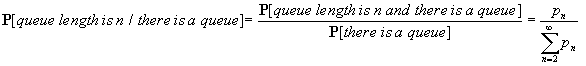
In (20) we have used the fact, that the second sum is a complement to p₀ and (17). Note, that (20) may be also used to compute L_Q provided L_S is known or vice versa. It is also possible to find an average queue length L_QQ provided there is a queue. For this we need the conditional probability p_n/q = P[queue length is n / there is a queue]. To find the conditional probability, let’s use the general formula:

that looks in our case like that (for n ³ 2):

Using the above formula for p_n/q , we may find L_QQ:

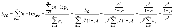
    (21)

The average queue length is a parameter that represents the quality of service especially from user’s point of view. Another parameters we need is the average time W_S spent in the system and the average time W_Q spent in the queue. These parameters are necessary to compute costs caused by customers waiting for service. There is a very important the so called Little’s formula, that gives the relation between the average number of customers in the system L_S and the average time W_S spent in the system and between the average number of customers in the queue L_Q and the average time W_Q spent in the queue:

L_S = l W_S        L_Q = l W_Q        (22,23)

This is the justification (not the exact proof) of the formula (22): let’s assume the average time spent in the system is W_S. During this time the average number of newcomers is W_Sl, because l is the arrival rate (average number of arrivals per time unit). So at the instant a customer is leaving the systems, it sees (on the average) W_Sl customers left in the system. Because in the stable state the average number of customers in the system is L_S, we have the above formula. Similar justification can be given for L_Q and W_Q (average number of arrivals during the time spent in the queue is lW_Q, that is the average number left in the queue when leaving the queue, that is L_Q). Using the Little’s formula we get these formulae:

         (24,25)

There is another obvious relationship between the average time spent in the system and the average time spent in the queue, because the total time spent is made of the time in the queue (that may be zero) and the time of the service:

    (26)

(26) can also be obtained from (24). Using the Little’s formula, it is possible to express a similar relation between L_S and L_Q by multiplying both sides of (26) by l :

    (27)

L_SERV = r is the average number of customers being served (that of course must be less than one). For a customer it is also important to know the probability, that the time spent in the system (or in the queue) will be greater than a certain value. Together with the queue length this probability represents a quality of service from user’s point of view. Without proof (that is less trivial) these formulae may be used:

     (28)

Of course the probabilities of spending less than t in the system (or in the queue) are complements of the above values to 1. Because the time spent is a continuous random variable, the probability of spending exactly the time t in system (queue) is zero, but using the formulae (28), we can compute the probability, that the time spent will be in certain range (t₁, t₂):

P[spending more than t₁ and less than t₂] = P[more than t₁] - P[more than t₂]

And finally the variances (squares of standard deviations) of the four characteristics:

         (29)