INTRODUCTION TO OOP IN SIMULA
©
1997 J.Sklenar (jaroslav.sklenar@um.edu.mt)
This document is based on an IT seminar called 30
Years of Object Oriented Programming (OOP) held at the University of Malta
on 5/12/1997. The first Object Oriented Language (OOL) Simula 67
was officially introduced by Ole Johan Dahl and Kristen Nygaard
at the IFIP TC 2 Working Conference on Simulation Languages in Lysebu near Oslo
in May 1967. 30 years represent one human and several computer generations. In
spite of being in use for such a long time, all modern programming work carried
out today is based on principles of OOP introduced for the first time in the
Simula definition. And what is more important, Simula contains facilities that
up to now have not been fully utilized and not even understood by not only
general programming public but also people from OOP community. The purpose of
the talk was a brief introduction of main Simula features, mainly those not
present in other OOLs. The same is the purpose of this document.
Notes:
- In
the following text the term object means a class instance
(note that "objects" of Object Pascal and some other OOLs are in
fact classes).
- You
can download all programs (simprogs.zip)
given in this document and some more. There is also a Turbo Pascal unit
SIMSET.PAS very similar to Simset of Simula. Use it if you want to work with
data structures with varying number of items. Expand the zip file in some
directory, where you will find a list of programs together with a brief
description in the file Readme.
- If
you are new in Simulation, consider browsing the page Simulation that explains the basic ideas of
computer simulation.
SIMULA PACKAGES = NESTED CLASSES
Go back to Author's home page
SIMULA - BASIC FACTS
Simula I = Process oriented discrete
simulation language based on Algol 60. (1964 - 1965) Simulation language.
Simula 67 = General object oriented language with system classes supporting linked
lists (the system class Simset) and discrete process oriented simulation (the
system class Simulation). (1967 - 1971) Simple universal language.
Simula = Simula 67 (The number is not used any more,
because Simula I has not been used for a very long time).
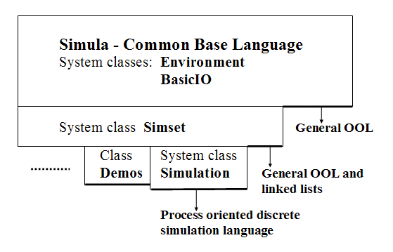
Figure
1: Main parts and interface lines in the Simula environment.
SIMULA I HISTORY
(Source: Jan Rune Holmevik:
Compiling Simula - see REFERENCES)
1952 Kristen Nygaard starts
work in Operations Research including writing simulation models. Problem: how to
conceptualize complex real world. Since the very beginning Simula intended to
be both system description and programming language.
1960 Algol 60 with its true
recursive block mechanism structure based on stack principle. All
important control structures introduced. Simula intended as a package
with preprocessor to Algol 60.
1962 Ole-Johan Dahl and
Kristen Nygaard meet in Norwegian Computing Center (NCC) in Oslo. First formal
language proposal presented at the IFIP 62 World Congress in Munich.
1962 Simula project
supported by UNIVAC, that resulted in UNIVAC 1107 installation in NCC in 1963.
1963 Conflict between
strict Algol stack mechanism and Simula's sophisticated simulation facilities
oriented more to queue principle. Preprocessor idea abandoned, Simula to
be an independent Algol based language.
1963 Ole-Johan Dahl works
on a new storage allocation scheme based on a two dimensional
list of free areas.
1964 Original idea of
passive customers moving through a network of active components (activity
approach) became a limiting factor. Other way round
possible - active customers moving through a passive network. This resulted in
a unifying general process concept:
System
= set of interacting quasiparallel processes.
1964 First prototype of
Simula compiler running on NCC's UNIVAC 1107 in December, Simula I manual
appeared in May 1965. During the first year Simula applied to a wide area of
Operations Research problems.
SIMULA 67 HISTORY
(Source: Jan Rune Holmevik:
Compiling Simula - see REFERENCES)
1965,66 Simula I used in
Sweden, Germany, USA (Burroughs B5500), Soviet Union (URAL 16) and other
countries. Effort to introduce and teach the language.
1965 Tony Hoare's
record class concept presented in Algol bulletin. After a careful
examination, Nygaard and Dahl accept the ideas, but a sort of generalized
concept still missing.
1966 Introducing the idea
of prefixing. Processes (later objects) made of two layers:
prefix layer, main layer. Idea of subclasses. Nygaard and Dahl
start work on a new general high-level language.
1967 (May). Simula 67
officially introduced by Dahl and Nygaard at the IFIP TC 2 Working
Conference on Simulation Languages in Lysebu near Oslo.
1967 (June). Definition of
Simula 67 standard called Common Base Standard.
1968 First meeting of
Simula Standards Group (SSG). After accepting string handling and I/O done by
Bjorn Myhrhaug, Simula formally frozen.
1973 Association of Simula
Users (ASU) founded. Simula used in more than 250 sites that year.
Implementations:
1969 CDC 3300, 3600 (Norway
- University of Oslo, NDRE)
1971 UNIVAC 1100 (NCC)
1972 IBM 360/370 (NCC)
1972 CII 10070, IRIS 80
(France)
1973/74 CDC 6000 (France,
Netherlands), CDC Cyber 70 (NDRE)
1975 DEC 10 (Sweden)
etc.
Periodicals:
Proceedings of annual ASU
conferences (first 1973 Oslo)
ASU Newsletter
SIMULA DATA TYPES
Simula contains all common facilities of high level
third generation languages. That's why the next two chapters are very brief
summaries, text being the only exception.
Value Types
Integer
Short Integer
Real Long Real
Boolean Character
Reference Types
Object Reference Declaration: Ref(
Object Identifier) (None is the trivial value)
Text Constants: "A", "Simula",
Notext
Text is conceptually
a class instance, that has its attributes and methods.
Methods:
Boolean Procedure Constant; (True if constant)
Text Procedure Main; (Main string - the text is a part of Main)
Integer Procedure Start; (Starting position in Main)
Integer Procedure Length; (Number of characters)
Integer Procedure Pos; (Current position)
Procedure SetPos(i); Integer i; (Changing position)
Boolean Procedure More; (True if Pos <= Length)
Character Procedure GetChar; (Character from Pos)
Procedure PutChar(c); Character c; (Storing character to Pos)
Text Procedure Sub(i, n); Integer i,n; (Substring at i of length n)
Text Procedure Strip; (Removes right spaces)
De-editing Methods:
Integer Procedure GetInt; (Reads integer)
Long Real Procedure GetReal; (Reads real)
Integer Procedure GetFrac; (Like GetInt, ignores spaces)
Editing methods:
Procedure PutInt(i); Integer i; (Writes integer value)
Procedure PutFix(i, n); Integer i,n; (Writes decimal value)
Procedure PutReal(r, n); Long Real r; Integer n; (Writes in scientific
format)
Procedure PutFrac(i, n); Integer i,n; (Groups of 3, spaces)
Text generation:
Text Procedure Blanks(n); Integer n; (Returns n blanks)
Text Procedure Copy(T); Text T; (Returns a copy of T)
Arrays
Examples of arrays
declared in blocks (n, m, a, b are global variables):
Integer Array MyList (1:100);
Array Matrix (1:n, 1:m); (Implicit type is real)
Character Array Buffer(1: If a>b then a else b);
SIMULA STATEMENTS
Simple statements
Assignment :=
Examples: X := If a>b Then a Else b ; X:=Y:=0; ( **
available )
Reference Assignment
:-
Examples: Queue :- New Head; T :- Blanks(80);
Procedure
Go to Goto
Structured statements
Begin ... End;
If ... Then ... ; If ... Then ...
Else ... ;
Switch Example:
Switch Target := L1, L2, L3, ... ;
Goto Target( Index_expression );
L1: ...
L2: ...
While ... do ... ;
For (very general) Example:
Begin
Integer i;
For i:= 1, 13, 20 step 10 until 40, 70, i+1 while i lt 76,
100 step 50 until 250, 1000, 1500 do OutInt(i,5);
End;
Output: 1 13 20 30 40 70 71 72 73 74 75 100 150 200 250
1000 1500
SIMULA PROCEDURES
Parameter Passing Modes:
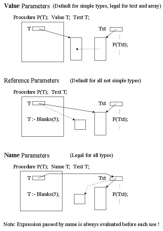
Figure 2: Parameter passing modes applied to a text parameter.
Procedures
Example procedure with two input and
one output parameters: (Displays a right indented text)
Begin
Procedure RightText(T, N, FitsIn); Text T; Integer N;
Name FitsIn; Boolean FitsIn;
Begin
Integer I;
FitsIn := N >= T.Length;
For i:=1 step 1 until N-T.Length do OutText(" ");
OutText(T)
End of RightText;
RightText("Short", 30); OutImage;
RightText("And the long one", 30);
End of Program;
Output:
Short And the long one
Functions = Type Procedures
Example integer function with two
input parameters: (Computes the greatest common divisor)
Begin
Integer Procedure GCD(M, N); Integer M, N;
Begin
While M<>N do
If M<N then N := N - M else M := M - N;
GCD := M
End of GCD;
Integer A, B;
OutText("Enter an integer number: "); OutImage; A := InInt;
OutText("Enter an integer number: "); OutImage; B := InInt;
OutText("Greatest Common Divisor of your numbers is ");
OutInt(GCD(A,B), 4); OutImage;
End of Program;
Note: A function may be called as if
it were a typeless procedure.
SIMULA CLASSES
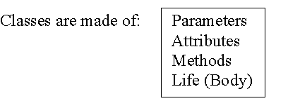
Figure 3: Simula classes are made of four parts.
Declaration:
Class Rectangle (Width, Height); Real Width, Height;
! Class with two parameters;
Begin
Real Area, Perimeter; ! Attributes;
Procedure Update; ! Methods (Can be Virtual);
Begin
Area := Width * Height;
Perimeter := 2*(Width + Height)
End of Update;
Boolean Procedure IsSquare;
IsSquare := Width=Height;
Update; ! Life of rectangle started at creation;
OutText("Rectangle created: "); OutFix(Width,2,6);
OutFix(Height,2,6); OutImage
End of Rectangle;
Object Generation:
Ref(Rectangle) R; (Class reference variable)
...
R :- New Rectangle(50, 40); Activities involved in this object
generation:
Memory allocation, reference stored to R.
Copying values to parameters (value passing only).
Starting the object's body (life rules).
Declaration of Subclasses:
Rectangle Class LocRectangle (X, Y); Integer X, Y;
Begin ! More parameters;
Boolean Tall; ! More attributes;
Procedure Move (Dx, Dy); Integer Dx, Dy; ! More methods;
Begin
X := X + Dx; Y := Y + Dy
End of Move;
! Additional life rules;
Tall := Height > Width;
OutText("Located at: "); OutFix(X,2,6); OutFix(Y,2,6); OutImage
End of LocRectangle;
Object Generation:
Ref(Rectangle) R; (Class reference variables)
Ref(LocRectangle) LR;
...
R :- New Rectangle(50, 40);
LR :- New LocRectangle(20, 30, 100, 200); (Note that also parameters for
the parent class are given)
Activities involved in the above
object generation:
Memory allocation, reference stored to LR.
Copying values to all parameters (parent class first).
Starting the body of the parent class, then the subclass.
This can be generalized to prefix sequence of
any length:
Class A; Begin ... LifeA End;
A Class B; Begin ... LifeB End;
B Class C; Begin ... LifeC End;
Ref(C) X;
...
X :- New C;
If not changed by Inner
- see next paragraph, the sequence of activities involved in the above object
generation is:
LifeA LifeB LifeC
Breaking life rules by the statement
Inner:
Example declarations:
Class A; Begin LifeA1 Inner; LifeA2
End;
A Class B; Begin LifeB1 Inner; LifeB2 End;
B Class C; Begin LifeC1 Inner; LifeC2 End;
Ref(C) X;
X :- New C;
The sequence of activities involved
in the above object generation is:
LifeA1 LifeB1 LifeC1 (Inner
in the life of C ignored) LifeC2 LifeB2 LifeA2
Notes:
1) Missing Inner is the same as Inner just before the class end.
2) Mostly one Inner is allowed in the class body.
Prefixing blocks:
Let's assume a program with the
following structure:
Begin
Class A(P); Integer P;
Begin LifeA1 Inner; LifeA2 End;
Part1
A(3) Begin
Block body
End;
Part2
End;
Activities involved in the execution
of the above prefixed block:
Creating a class instance of A.
Copying values to its parameter(s).
Starting the body of the class, that includes execution of the block code.
So in the above program the sequence
of operations is this:
Part1 LifeA1 Block body LifeA2 Part2
Prefixed block is conceptually
a class instance without a name that has:
- parameters of the prefix
class
- more attributes (class
attributes + local block variables)
- more methods (class methods
+ local block procedures)
- more complex life rules
(class body + block body).
Notes:
1) Block prefixing mechanism is not very useful in case of simple
classes. The possible use is import of class declarations (parameters,
attributes, and methods) into the block. It is supposed to be used mainly with
the main classes (see the next chapter), that represent modules created
by OOP principles. Prefixing a block by a main class (like for example
Simulation) may import whole programming environments or special purpose Simula
based languages.
2) In Simula programs there is no explicit memory deallocation because
the Garbage Collector recovers automatically the memory occupied
by not referenced class instances.
Navigation in the prefix sequence
The following text is based on these
declarations:
Class A; Begin Ref(A) Link;
Procedure Show; ... End;
A Class B; Begin Procedure Show; ... End;
B Class C; Begin Procedure Show; ... End;
Ref(A) XA, First, Current; Ref(B)
XB; Ref(C) XC;
1. Qualification by the Inspect statement
a) Simple
Inspect XA do Show; does basically the same as XA.Show;
The difference is that with Inspect
if XA = None, the statement after do is ignored. If XA = None, XA.Show
results in a run time error.
b) Testing None by the clause Otherwise
Inspect XA do Begin
Show; ...
End
Otherwise Begin
OutText("Sorry, XA not created"); OutImage
End;
c) Testing type by the clause When
Displaying a linked list made of various
items of types A, B, and C, whose head pointer is in First:
Current :- First;
While Current ne None do begin
Inspect Current
When A do Show ! Show of A;
When B do Show ! Show of B;
When C do Show ! Show of C;
Otherwise OutText("Not a (sub)class of A");
OutImage;
Current :- Current.Link
End While;
2. Instantaneous Qualification by
the Qua clause
Assume these statements based on the
above declarations:
XA :- New B; XB :- New B;
XA.Show; ! Show of A;
XA Qua B.Show; ! Show of B - it is possible to go down;
XB Qua A.Show; ! Show of A - it is possible to go up;
XA :- New A;
XA Qua B.Show; ! This is illegal - attributes of B do not exist;
Note: Normal properties of a reference variable
qualified to B declared as Ref(B) XB :
- Can
not reference objects of class A.
- Can
reference objects of class B, that allows access to attributes of B and
those of A not re-declared in B.
- Can
reference objects of class C, but only attributes of B and not re-declared
attributes of A can be accessed.
These normal properties can be overcome by Inspect or Qua.
Note from the third rule that the usual late binding mechanism (as for
example in Object Pascal) does not work automatically in Simula.
Solution to this problem is Inspect with When clauses - see the
above example. Simula's approach is maybe less user friendly, but it is more
general and the programmer has everything under control.
3. Referencing itself by This
The following code is a method of A
that adds the object to the list First:
Procedure Add_to_List(First); Name First; Ref(A) First;
Begin
Link :- First; First :- This A
End;
4. Testing Qualification by Is and In
The following selfexplaining code segments based on the declarations Ref(B)
XB and Ref(A) XA show a use of the very user friendly operators Is
and In. Note that for example Object Pascal does not have en
equivalent of In. The only solution to this problem in Object
Pascal is implementation of methods that return identification of ancestors.
If XB is B then
OutText("XB is B")
Else
OutText("XB is either subclass of B or None");
If XA in B then
OutText("XA is either B or its subclass")
Else
OutText("XA is either A or None");
5. Protecting attributes
Hidden attributes can be used only in the
body of the class where they are declared.
Protected attributes can be used only in
bodies of the class where they are declared and all subclasses.
SIMULA PACKAGES = NESTED CLASSES

Figure 4: Simula classes can be nested to any depth.
Classes that contain declaration of local classes are called main
classes. Next example code defines a main class called Geometry.
! The program defines the main class "Geometry". ;
! It represents a theory with terms "point, rectangle, circle, and line".;
Class Geometry;
Begin
Class Point(X,Y); Real X,Y;
Begin
Procedure Print; Begin ... End;
Procedure Shift(Dx, Dy); Real Dx, Dy; Begin ... End;
Print; ! Life of point;
End of Point;
Class Rectangle(RecName, Width, Height);
Text RecName; Real Width, Height;
Begin
Real Area, Perimeter;
Procedure Update; Begin ... End;
Procedure Show; Begin ... End;
Update; Show; ! Life of rectangle;
End of Rectangle;
Class Circle(Radius, Center); Real Radius; Ref(Point) Center;
Begin
Procedure Shift(Dx, Dy); Real Dx, Dy; Begin ... End;
OutText("Circle created at "); ! Life of circle;
Center.Print;
End of Circle;
Class Line(M,N); Ref(Point) M,N; ! Line defined by two points;
Begin
Real Slope;
Slope := ... ; ! Life of line;
End of Line;
!Variables declared in geometry: ;
Ref(Point) Origin, A, B;
Ref(Line) X,Y;
!Life of geometry: ;
Origin :- New Point(0,0); ! Creating the origin;
A :- New Point(1,0); B :- New Point(0,1);
X :- New Line(Origin, A); ! Creating the axes;
Y :- New Line(Origin, B);
OutText("*** Geometry initialized ***"); OutImage;
End of Geometry;
Next program is using the main class Geometry. Note how the classes
declared in Geometry are used to declare subclasses specialized to the problem
being solved. Later it is possible to declare and use reference variables
qualified into both imported and locally declared classes. This is the
fundamental idea of Simula based packages or user defined languages (what is
the difference?)
External Class Geometry;
Geometry Begin
! Subclasses declared in the prefixed block: ;
Point Class Color_Point(C); Character C; Begin ... End;
Rectangle Class Square; Begin ... End;
! Variables declared in the prefixed block: ;
Ref(Color_Point) A1;
Ref(Point) C, D;
Ref(Circle) K;
Ref(Line) E, F;
Ref(Rectangle) R1;
Ref(Square) S1;
! Block body: ;
C :- New Point(5,6);
D :- New Point(20,30);
A1 :- New Color_Point(3, 4, 'G');
K :- New Circle(10, C);
E :- New Line(C, D);
F :- X;
K.Shift (1,1);
R1 :- New Rectangle("Rec_R1", 5, 4);
S1 :- New Square("Square_S1", 4, 6);
S1.Show;
End of prefixed block;
SIMULA STANDARD PACKAGES
Environment -
the system facilities
Attributes are available for:
- Environmental
constants (MaxInt, MaxReal, ... )
Methods are available for:
- Basic
arithmetical operations (Mod, Abs, ... )
- Basic
text and character handling (Copy, Blanks, UpCase, ... )
- Mathematical
functions (Sin, Exp, ... )
- Extreme
functions (Max, Min)
- Random
numbers (Draw, Uniform, Normal, Histo, ... )
- Compiler
information (SourceLine, SIMULAId)
- Others
(Error, Upper/LowerBound of arrays, Date, Time, ... )
BasicIO - the world outside
All input and output operations are represented by methods of file
objects. A common ancestor called File - see Figure 5 - implements
facilities common to all files. Its subclasses are ByteFile and ImageFile
(text file - "image" is its text buffer). Both are further
specialized according to the access method (input, output, direct access). OutFile
has one more descendent PrintFile that implements page oriented text
output. Note that Simula does not have typed files made of for example records.
This type of files can be implemented by byte files. Figure 5 contains some
more important methods with selfexplaining names.
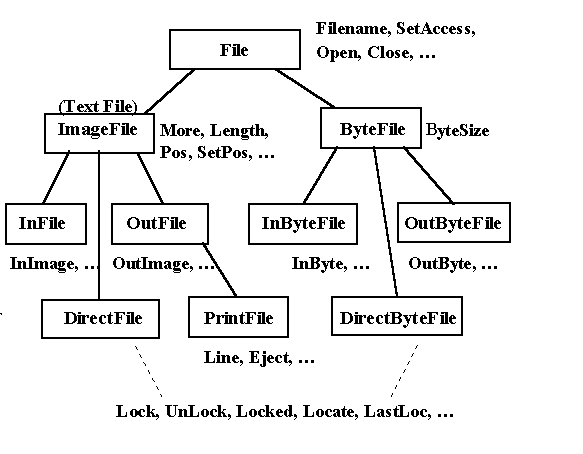
Figure 5: Hierarchy of Simula file classes.
Program frame
All system facilities in Simula are conceptually implemented as classes
with certain attributes, methods and local classes. User programs are written
as if they were inserted into the following frame. Note that the life rules of
the class BasicIO create and open the system files before starting the
user code. After its termination the system files are closed. The user code is
inserted into a double Inspect statement. It means, that methods of system
files (like for example GetInt, OutImage, etc.) need not be preceded by the
file name.
Begin
Class Environment; ...
Environment Class BasicIO ... ;
Begin
Ref(InFile) SysIn; Ref(OutFile) SysOut; ...
Class Simset ... ;
Simset Class Simulation ... ;
Procedure Terminate_Program;
Begin ... ; GoTo STOP End;
...
SysIn :- New InFile ( ... );
SysOut :- New PrintFile ( ... );
SysIn.Open ( ... );
SysOut.Open ( ... );
Inner; ! This starts the user program;
STOP: SysIn.Close ( ... );
SysOut.Close ( ... )
End BasicIO;
BasicIO Begin
Inspect SysIn do
Inspect SysOut do
Begin ! User program starts by this begin;
User statements
End; ! Last line of user program;
End;
End;
Simset - the world of linked lists
The system class Simset implements circular two-way linked
lists with the head item involved in the linking, that were originally called
"sets" - see Figure 6.

Figure 6: Simula linked lists implemented in the system class Simset.
The above lists are represented by three classes - see Figure 7. Linkage
is a knowledge about two way linking as such. This is further specialized as a
header and a member elements.
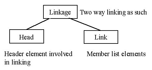
Figure 7: Classes declared in the system class Simset.
Methods of list related classes:
Linkage
- Suc
is the successor qualified to Link (None for the
last item of the list).
- Pred is the predecessor qualified to Link (None for the first item of
the list).
- Prev is the previous item qualified to Linkage.
Head
- First is the first item of the list (None if the list is empty).
- Last is the last item of the list (None if the list is empty).
- Empty
returns true if the list is empty.
- Cardinal is the number of items in the list.
- Clear removes all items from the list, memory will be recovered by the
garbage collector.
Link
- Into(S) inserts the item at the end of the list (Head) S.
- Out removes the item from the list.
- Follow(L)
inserts the item that performs this method after
the Linkage L.
- Precede(L) inserts the item that performs this method before the Linkage L.
Methods can be combined to represent complex activities. For example the
procedure statement:
Queue1.Last.Precede(Queue2.First);
removes the last item from Queue1
and inserts it at the beginning of Queue2.
SIMULA QUASIPARALLEL SYSTEMS
Life rules of Simula objects are coroutines, that may be temporarily stopped
and later resumed. There are two levels of (quasi)parallelism in Simula. First
level does not work with time, the programmer "thinks in
quasiparallel". The second level introduces the notion of time, the
programmer works with parallel (from user's point of view) processes. First
level can be applied to all classes, the second level is implemented by the
class Process of the system class Simulation.
Figure 8 shows the possible states of a coroutine (body) of an object X.
Note that a coroutine that does not use any of the next facilities is at first attached,
then terminated (objects of other OOLs are always terminated). A
terminated object can still be used (it is possible to call its methods and/or
to access its attributes). These are the Simula facilities (methods available
in all classes) that support work with quasiparallel systems (QPS):
Detach stops the execution of the current object (the one that performs
Detach). The current object becomes detached. Control is passed
to the point where the current object was either created or resumed.
Resume(Y) activates a detached object Y that becomes resumed. The
current object becomes detached.
Call(Y) is similar to Resume, but the object Y becomes attached to the current
object. The current object becomes detached. The current object will be resumed
after detaching Y.
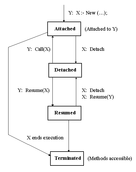
Figure 8: State diagram of Simula coroutines.
QPS Example 1:
Chess game control using Two Masters approach.
In the following program there are three coroutines: the two players and
the main block. Note that the first two moves are special. A player can win with
certain probability from the third move onwards: Draw(0.3,Seed) is a boolean function that returns true with the probability 0.3. Note how
the main block creates the two players, links them by the attributes Opponent
and passes control to the White. Then the players repeatedly make their
moves and resume the opponent until one of them wins. This terminates their
bodies and the control is passed to the main block.
Begin
Boolean Mate;
Ref(Player) White, Black, Winner;
Integer Seed;
Class Player(PName); Text PName;
Begin
Ref(Player) Opponent;
Integer Move;
! The life follows;
Detach;
OutText(PName); OutText("'s First Move"); OutImage;
Resume(Opponent);
OutText(PName); OutText("'s Second Move"); OutImage;
Resume(Opponent);
Move := 2;
While not Mate do begin
Move := Move+1;
OutText(PName); OutText("'s Move # ");
OutInt(Move,3); OutImage;
If Draw(0.3,Seed) then begin
Mate := true; Winner :- This Player;
End If;
Resume(Opponent);
End While;
End of Player;
Begin ! QPS head;
OutText("Creating Players, Starting the white one"); OutImage;
White :- New Player("White");
Black :- New Player("Black");
White.Opponent :- Black;
Black.Opponent :- White;
Seed := 17;
Resume(White);
OutText("Finish: "); OutText(Winner.PName);
OutText(" won in move"); OutInt(Winner.Move,3); OutImage;
End of QPS
End of program;
This is the indented output of the above program. Indentation shows the
object, that generates the output - from left: Main block, White, Black.
Creating Players, Starting the white one
White's First Move
Black's First Move
White's Second Move
Black's Second Move
White's Move # 3
Black's Move # 3
White's Move # 4
Black's Move # 4
Finish: Black won in move 4
QPS Example 2:
Chess game control using Master and Two Slaves approach.
In the following program there are also three coroutines: the two
players and the main block. The difference between this and the previous
program is the active role of the main block. Players do not resume each other.
They just make the move and detach. The main block activates them repeatedly
until one of them wins. Note the use of Call - the players are
repeatedly attached to the main block.
Begin
Boolean Mate;
Ref(Player) White,Black,Winner;
Integer Seed;
Class Player(PName); Text PName;
Begin
Ref(Player) Opponent;
Integer Move;
! The life follows;
Detach;
OutText(PName); OutText("'s First Move"); OutImage;
Detach;
OutText(PName); OutText("'s Second Move"); OutImage;
Detach;
Move := 2;
While true do begin
Move := Move+1;
OutText(PName); OutText("'s Move # ");
OutInt(Move,3); OutImage;
If Draw(0.05,Seed) then begin
Mate := true; Winner :- This Player;
end;
Detach;
End While;
End Player;
Begin
OutText("Creating Players, Starting the game"); OutImage;
White :- New Player("White");
Black :- New Player("Black");
White.Opponent :- Black;
Black.Opponent :- White;
Seed := 11;
While not Mate do begin
Call(White);
If not Mate then Call(Black)
End While;
OutText("Finish: "); OutText(Winner.PName);
OutText(" won in move"); OutInt(Winner.Move,3); OutImage;
End
End;
This is the indented output of the above program. Indentation shows the
object, that generates the output - from left: Main block, White, Black.
Creating Players, Starting the game
White's First Move
Black's First Move
White's Second Move
Black's Second Move
White's Move # 3
Black's Move # 3
White's Move # 4
Black's Move # 4
White's Move # 5
Black's Move # 5
White's Move # 6
Finish: White won in move 6
QPS Example 3:
Chess game control using Master and Two Slaves approach implemented as a
package (main class).
In the following program the main class Chess declares two
local classes: Player and Referee. The life rules
of the main class prepare the game by creating and linking the two players and
the referee. All three objects detach and the body of the main class
terminates. The game must be started by the program (a block prefixed by
Chess). Prefixing imports all declarations and prepares the game. Note, that
the prefixed block just activates the referee and evaluates the game.
Class Chess; ! Main class with local: Player, Referee;
Begin
Boolean Mate;
Ref(Player) White,Black,Winner;
Ref(Referee) Master;
Integer Seed;
Class Player(PName); Text PName;
Begin
Ref(Player) Opponent;
Integer Move;
! The life of Player;
Detach;
OutText(PName); OutText("'s First Move"); OutImage;
Detach;
OutText(PName); OutText("'s Second Move"); OutImage;
Detach;
Move := 2;
While true do begin
Move := Move+1;
OutText(PName); OutText("'s Move # ");
OutInt(Move,3); OutImage;
If Draw(0.05,Seed) then begin
Mate := true; Winner :- This Player;
end;
Detach;
End While;
End Player;
Class Referee;
Begin
Detach;
While not Mate do begin
Call(White);
If not Mate then Call(Black)
End While
End of Referee;
Begin ! Life of Chess;
Seed := 11;
OutText("Creating the Players and the Master"); OutImage;
White :- New Player("White");
Black :- New Player("Black");
White.Opponent :- Black;
Black.Opponent :- White;
Master :- New Referee;
End
End of Chess;
The next program uses the main class Chess:
External Class Chess;
Chess Begin
OutText("Resuming the Master"); OutImage;
Resume(Master);
OutText("Finish: "); OutText(Winner.PName);
OutText(" won in move"); OutInt(Winner.Move,3); OutImage;
End of Program;
This is the indented output of the above program. Indentation shows the
object, that generates the output - from left: Body of Chess, Prefixed
block, White, Black.
Creating the Players and the Master
Resuming the Master
White's First Move
Black's First Move
White's Second Move
Black's Second Move
White's Move # 3
Black's Move # 3
White's Move # 4
Black's Move # 4
White's Move # 5
Black's Move # 5
White's Move # 6
Finish: White won in move 6
SIMULATION = WORLD OF PARALLEL PROCESSES
The basic notion of the system class Simulation is Process
- sequence of instantaneous events (represented by code segments) separated by
passive periods. Figure 9 shows the classes declared in Simulation and their
methods. Event Notice (a subclass of Link) represents a scheduled
event that will occur in certain time - EvTime - in future. Proc
is the process whose code segment will be activated. SQS (a
subclass of Head) is a list of events ordered by time. It is the usual Calendar
of discrete simulation languages. Conceptually it an ordered linked list,
internal implementation is typically based on a more efficient tree structure.
Obviously this list can not be accessed directly from the user program. There
are scheduling facilities - see later, that support work with time and mutual
synchronization of processes. Processes of the user program are subclasses of
the common ancestor Process. The first two methods test its
status, the other two return the next scheduled event and its activation time.
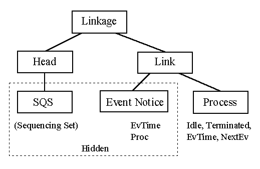
Figure 9: Classes of the system class Simulation.
Facilities of the system class Simulation are implemented by the
"low level" quasiparallel methods: detach, resume, call, but they are
more user friendly. A user of Simulation "thinks in parallel".
Dynamics of a simulation model is expressed in terms of mutually interacting
parallel processes. This way is very natural - it is exactly how real world
works.
States of a process object:
- Active a segment of the process is being executed.
- Suspended
process has its event notice in SQS. Unless
canceled it will be activated in future.
- Passive
process has no scheduled event. It must be
activated by another process.
- Terminated
process has finished. It can not be activated
again.
Timing, Sequencing and Synchronizing Facilities:
- Activate
X activates a passive process X.
- Reactivate X. either activates a passive process or changes the next
activation time if the process is suspended or active.
- Hold(T) generates the delay T in the process life.
- Passivate
makes the current process passive.
- Cancel(X) cancels the next activation of X.
- Wait(Q) passivates the process and puts it at the end of the list
(queue) Q.
Simulation Example 1: A
multichannel queuing system - Active Customer approach.
Figure 10 shows the system being simulated. It is an abstraction of for
example a bank where the customers wait in one queue for any of the tellers.
The interval between arrivals is random, uniformly distributed between 1 to 3
minutes. All servers have the same random service time, that is normally
distributed with the mean value 8 minutes and the standard deviation 2 minutes.
The simulation should find the average time a customer spends in the system.
(Note, that an analytical model of the above system is not available).
Simulation of similar systems in Simula (exactly in the system class Simulation
of Simula) always starts by identification of processes. One process is
obviously the generator of customers - it will repeatedly generate a customer,
record its arrival time, and wait a random delay. To express the dynamics of
the system, there are two logical approaches. First (used in this example) is
based on active customers and passive servers. The opposite approach - active
servers, passive customers is shown in the next example. An active
customer has life rules represented by the following
steps:
- If
there is a free server, proceed. Wait in the queue otherwise.
- Seize
a server, generate random delay, that represents the service time.
- Release
the server.
- If
there is a waiting customer (if the queue is not empty), remove it from
the queue and activate it. (The activated customer will start its step 2.)
- Update
statistics.
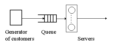
Figure 10: Queuing system made of one queue and more servers.
The following program is a simulation model of the above system. Note,
that the primary objective was to show the logic of the model in a program as
simple as possible. Real simulation models of course prompt for all variable
parameters and provide more results (like for example average and maximum queue
length, etc). In the following program there are two processes that exist
during the whole experiment: the generator and the main program (block prefixed
by Simulation), that just waits until the experiment is over and then displays
the result. Then there is a varying number of customer processes, that exist
temporarily. After updating statistics the customers terminate. Note the use of
standard functions to generate random delays. There are standard functions in
Simula for most commonly used distributions. All are given an integer variable
as a seed to be used by the random generator. So all random values may use
separate streams of random numbers or share a common one.
! Active customer approach;
Simulation Begin
Real TrialDuration; ! Experiment length [min];
Ref(Head) Queue; ! The queue;
Integer Servers; ! Total number of servers;
Integer BusyServers; ! Numbers of working servers;
Integer TrialSeedG, TrialSeedS; ! Seeds of random generators;
Long Real TotalTime, TimeSpent; ! Variables for statistics;
Integer CustomersOut; ! Number of served customers;
Real MinInt, MaxInt; ! Uniform interval between arrivals;
Real SMean, SStd; ! Normal service duration;
Process Class Generator;
Begin
While true do begin
Activate New Customer(Time); ! Time is the current (arrival) time;
! Interval between arrivals: ;
Hold(Uniform(MinInt, MaxInt, TrialSeedG));
End While;
End of Generator;
Process Class Customer(Arrival); Real Arrival;
Begin
Ref(Customer) Next;
If not Queue.Empty or (BusyServers >= Servers) then
Wait(Queue); ! Customer has to wait in the Queue;
! Service can start: ;
BusyServers := BusyServers + 1; ! Seize a server;
! This is the teller service: ;
Hold(Normal(SMean, SStd, TrialSeedS));
BusyServers := BusyServers - 1; ! Release the server;
If not Queue.Empty then begin
Next :- Queue.First;
Next.Out; ! First from Queue served;
Activate Next after Current;
End If;
CustomersOut := CustomersOut + 1; ! Statistics;
TotalTime := TotalTime + (Time - Arrival);
End of Customer;
! MAIN program body: ;
TrialSeedG := 7; TrialSeedS := 23; ! Seeds for random variables;
MinInt := 1; MaxInt := 3; ! Min and Max intervals;
SMean := 8; SStd := 2; ! Random normal servers;
OutText("Enter the number of Servers : "); OutImage;
Servers := InInt; ! Initial numbers;
TrialDuration := 600; ! Other variables initialized to 0;
Queue :- New Head; ! Create an empty queue;
Activate New Generator; ! This starts the experiment;
Hold(TrialDuration); ! Experiment duration;
TimeSpent := TotalTime/CustomersOut;
OutText("Average time spent in the system: ");
OutFix(TimeSpent, 3, 10); OutImage;
InImage
End of program;
Simulation Example 2: A
multichannel queuing system - Active Server approach.
The system being simulated is the same, as in the previous example - see
Figure 10. The difference is the active server, that repeatedly serves
customers from the queue until the queue is empty. Then the server passivates.
Customers at first activate all idle servers (if any) and then go into the
queue. This is of course not very efficient, but simple. Customers are
activated by servers after completing the service. In the rest of their lives
the customers just update statistics. The main program creates and activates
all servers, but they immediately passivate, because the queue is empty. Then
the main program activates the generator and waits until the experiment is
over.
! Active server approach;
Simulation Begin
Real TrialDuration; ! Experiment length [min];
Ref(Head) Queue; ! The queue;
Integer Servers; ! Total number of servers;
Integer TrialSeedG, TrialSeedS; ! Seeds of random generators;
Long Real TotalTime, TimeSpent; ! Variables for statistics;
Integer CustomersOut; ! Number of served customers;
Real MinInt, MaxInt; ! Uniform interval between arrivals;
Real SMean, SStd; ! Normal service duration;
Ref(Server) Array ServBank(1:10); ! Max. number of servers is 10;
Integer i;
Process Class Generator;
Begin
While true do begin
Activate New Customer(Time);
! Interval between arrivals: ;
Hold(Uniform(MinInt, MaxInt, TrialSeedG));
End While;
End of Generator;
Process Class Server;
Begin
Ref(Customer) ServedOne;
While true do
If not Queue.Empty then begin
ServedOne :- Queue.First;
ServedOne.Out; ! First from Queue served;
Hold(Normal(SMean, SStd, TrialSeedS));
Activate ServedOne after Current
end
Else
Passivate;
End of Server;
Process Class Customer(Arrival); Real Arrival;
Begin
For i:=1 step 1 until Servers do
If ServBank(i).Idle then
Activate ServBank(i) after Current;
Wait(Queue);
! Service finished: ;
CustomersOut := CustomersOut + 1; ! Statistics;
TotalTime := TotalTime + Time - Arrival;
End of Customer;
! MAIN program body: ;
TrialSeedG := 7; TrialSeedS := 23; ! Seeds for random variables;
MinInt := 1; MaxInt := 3; ! Min and Max intervals;
SMean := 8; SStd := 2; ! Random normal servers;
OutText("Enter the number of Servers : "); OutImage;
Servers := InInt; ! Initial numbers;
TrialDuration := 600;
Queue :- New Head;
For i:=1 step 1 until Servers do begin
ServBank(i) :- New Server;
Activate ServBank(i) ! Create and activate all servers;
End For;
Activate New Generator; ! This starts the experiment;
Hold(TrialDuration); ! Experiment duration;
TimeSpent := TotalTime / CustomersOut;
OutText("Average time spent in the system: ");
OutFix(TimeSpent, 3, 10); OutImage;
InImage
End of program;
SIMULA NESTED QPS
A quasiparallel system (QPS) in Simula is basically a block (typically
but not necessarily a prefixed one), whose body creates some objects that
together with the main block made up the system of quasiparallel coroutines.
Because Simula (unlike for example Pascal) is a true block oriented language,
block (that generally means a QPS) can occur at any place in the code as a
statement. It means, that a QPS can contain local (nested) QPS's, that can also
contain local QPS's, etc. This simple rule gives a way to create incredibly
complex structures with consequences, that so far have not been fully utilized
and not even understood. The next program outlines a possible use of a nested
QPS in the chess control. Next chapter shows a simulation program with nested simulation.
Nested QPS Example: A
chess control using simulated game as a part of decision.
Let's assume that a chess player as a part of his/her decision simulates
the current game to check the possible outcome of the next move. The following
program (based on the Two Masters approach) is an outline of one possible
solution. Note that the class Player has a method TestStrategy
called as a part of each decision. This method implements a QPS similar
to the outer one. It contains a local class TestPlayer, that
might be very similar to the outer Player, except TestStrategy
(it can have something similar, but nesting has to stop at certain level). The
body of TestStrategy is the internal QPS whose results are used by
Player at the upper level.
Begin
Boolean Mate;
Ref(Player) White, Black, Winner;
Integer Seed;
Class Player(PName); Text PName;
Begin
Ref(Player) Opponent;
Integer Move;
Procedure TestStrategy;
Begin
Class TestPlayer ... ;
Begin
! Internal experiment, similar to the outer QPS;
...
End of internal QPS;
End of TestStrategy;
! The life of Player;
Detach;
TestStrategy;
OutText(PName); OutText("'s First Move"); OutImage;
Resume(Opponent);
TestStrategy;
OutText(PName); OutText("'s Second Move"); OutImage;
Resume(Opponent);
Move := 2;
While not Mate do begin
Move := Move+1;
TestStrategy;
OutText(PName); OutText("'s Move # ");
OutInt(Move,3); OutImage;
If Draw(0.3,Seed) then begin
Mate := true;
Winner :- This Player;
End If;
Resume(Opponent);
End While;
End of Player;
Begin ! This block is the outer QPS head;
OutText("Creating Players, Starting the white one"); OutImage;
White :- New Player("White");
Black :- New Player("Black");
White.Opponent :- Black;
Black.Opponent :- White;
Seed := 17;
Resume(White);
OutText("Finish: "); OutText(Winner.PName);
OutText(" won in move"); OutInt(Winner.Move,3); OutImage;
End of outer QPS;
End of program;
SIMULA NESTED SIMULATION
There are two levels of quasiparallelism in Simula, both can implement
nested systems. The previous chapter deals with low level nested QPS's. The
system class Simulation introduces the notion of time. It means that if nested,
there will be other local (nested) times. The basic idea is in the Figure 11.
The Hold statements with delays x and z apply to the main (outer)
time. The Hold statement with the delay y is in another alternative
world. So in Simula it is possible to simulate systems found so far only in
science fiction. There are practical applications. Basically it is possible to
simulate systems that contain simulation as a part of decision making. Consider
this situation: there is a certain complex system and a group of experts who
suggest different decisions, whose outcomes can not be tested in trivial or
analytical way. (Is not this the usual case in practice?) To test and evaluate
their decision proposals, the experts perform simulation experiments, compare
the results and select the most promising decision. Now suppose, that all this
will be simulated.
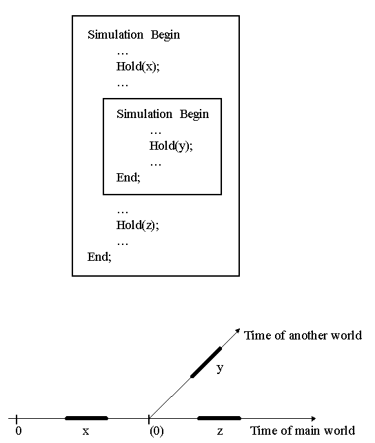
Figure 11: Basic ideas of Nested Simulation.
Nested Simulation Example: A queuing network whose part is optimized by repeated nested
simulation.
Figure 12 shows the system being simulated. It is an abstraction of for
example a bank where the customers at first wait in one queue for a teller.
After being served by a teller, a customer is served by a cashier. There is
another queue, where the customers wait for cashiers. The random interval
between arrivals and the random service times of tellers and cashiers are
known. Let's assume, that there is a certain number of clerks, that can work
both as tellers and as cashiers. The management of the bank wants to check the
way the clerks are allocated as tellers and as cashiers during a typical shift
made of three periods: busy, idle, and a very busy one with different intervals
between arrivals of customers. To find the best allocation policy, a nested simulation
can be used in this way: at the beginning of each period, the internal repeated
simulation will test the behavior of the first stage for various numbers of
tellers (obviously the range is from 1 to the total known number of clerks).
Using results from these internal simulation experiments, the management will
choose the number of clerks who will work as tellers, the others will work as
cashiers. To make the program simple, the decision is done by the user, who is
given the results of internal simulation and then prompted to enter the number
of tellers and the number of cashiers. The decision criterion is the average
time spent in the first stage. The policy as such is also evaluated by the
average time spent in the whole system.
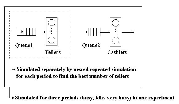
Figure 12: Queuing network made of two multichannel servers.
The following "program" is an outline of the simulation
program (that follows). Note, that the internal block prefixed by Simulation
is performed repeatedly three times for all possible numbers of tellers. It
contains declaration of classes similar to the outer ones. The difference is a
simpler behavior of the customer, because there is only one service stage.
There is also no further nesting. Basically the internal simulation is similar
to the example given in the chapter on the system class Simulation (active
customer approach).
Simulation Begin
Declaration of global variables
Process Class Generator; Begin ... End;
Process Class Customer; Begin ... End;
Initialize the global experiment
For Period:=1 step 1 until 3 do begin
For Trial:=1 step 1 until MaxClerks do
Simulation Begin
Declaration of internal global variables
Process Class Igenerator; Begin ... end;
Process Class Icustomer; Begin ... End;
Perform and evaluate one inner experiment
End of internal simulation;
Show results of internal experiments;
Select the best numbers of tellers and cashiers;
Perform a part of outer experiment for this period
End For;
Evaluate the global experiment
End of program;
The next program is the nested simulation
model with the above structure.
! NESTED Simulation using the Simula's class SIMULATION ;
! ;
! The example is a model of a bank. Customers are first ;
! served by tellers, then by cashiers. ;
! The input rate changes in three periods: there is a busy ;
! period, then an idle period and again a busy one. ;
! For each period the repeated inner simulation experiment ;
! simulates the first queue for the particular input rate ;
! and for various numbers of servers. Then it shows the ;
! results (average time spent at the first server) and ;
! prompts the user for the number of tellers and the number;
! of cashiers. Tellers always finish a service that has ;
! already started. The simulation should find the ;
! time customers spend in the bank (average and maximum) ;
! for various numbers of clerks in the three periods. ;
! ;
Simulation Begin
! Global variables: ;
Integer Period,Trial; ! Period, Trial number;
Real Array MinInt,MaxInt(1:3); ! Min and Max intervals;
Real Array Duration(1:3); ! Duration of periods [min];
Ref(Head) Queue1,Queue2; ! The two queues;
Integer MaxClerks, Tellers, Cashiers; ! Total numbers;
Integer BusyTellers, BusyCashiers; ! Numbers of working clerks;
Real S1Mean, S1Std, S2Mean, S2Std; ! Random normal servers;
Integer SeedG, SeedS1, SeedS2; ! Seeds of the random generators;
Long Real TotalTime, MaxTime; ! Variables for statistics;
Integer CustomersOut; ! Number of served customers;
Process Class Generator;
Begin
While true do begin
! Interval between arrivals: ;
Hold(Uniform(MinInt(Period),MaxInt(Period),SeedG));
Activate New Customer(Time);
End While;
End of Generator;
Process Class Customer(Arrival); Real Arrival;
Begin
Ref(Customer) Next;
Real Spent;
If (not Queue1.Empty) or (BusyTellers >= Tellers) then
Wait(Queue1); ! Has to wait in Queue1;
! Service can start;
BusyTellers := BusyTellers + 1;
Hold(Normal(S1Mean, S1Std, SeedS1)); ! This is the teller service;
BusyTellers := BusyTellers - 1;
If (not Queue1.Empty) and (BusyTellers < Tellers) then begin
Next :- Queue1.First;
Next.Out; ! First from Queue1 served;
Activate Next after Current;
End If;
If (not Queue2.Empty) or (BusyCashiers >= Cashiers) then
Wait(Queue2); ! Has to wait in Queue2;
! Service can start;
BusyCashiers := BusyCashiers + 1;
Hold(Normal(S2Mean, S2Std, SeedS2)); ! This is the cashier service;
BusyCashiers := BusyCashiers - 1;
If (not Queue2.Empty) and (BusyCashiers < Cashiers) then begin
Next :- Queue2.First;
Next.Out; ! First from Queue2 served;
Activate Next after Current;
End If;
CustomersOut := CustomersOut + 1;
Spent := Time - Arrival;
TotalTime := TotalTime + Spent;
If Spent > MaxTime then MaxTime := Spent;
End of Customer;
Procedure Report; ! Experiment evaluation;
Begin
OutText(" *** Report on external simulation ***"); OutImage;
OutInt(CustomersOut,6); OutText(" customers ready at time ");
OutFix(Time,2,10); OutImage;
OutText("Average time in system: ");
OutFix(TotalTime/CustomersOut,2,10); OutImage;
OutText("Maximum time in system: ");
OutFix(MaxTime,2,10); OutImage;
End of Report;
! MAIN program body;
SeedG := 11; ! Seeds of random variables;
SeedS1 := 13;
SeedS2 := 17;
MinInt(1) := 1; MaxInt(1) := 4; ! Min and Max intervals;
MinInt(2) := 2; MaxInt(2) := 9;
MinInt(3) := 1; MaxInt(3) := 3;
Duration(1) := 120; ! Duration of periods;
Duration(2) := 240;
Duration(3) := 120;
MaxClerks := 6;
S1Mean := 6; ! Random normal servers;
S1Std := 1;
S2Mean := 8;
S2Std := 2;
Queue1 :- New Head;
Queue2 :- New Head;
Period := 1;
Activate New Generator;
For Period:=1 step 1 until 3 do begin
Real Array TimeSpent(1:MaxClerks);
OutText(" *** Results of internal simulation *** Period ");
OutInt(Period,1); OutImage;
OutText(" Tellers Average time spent"); OutImage;
For Trial:=1 step 1 until MaxClerks do
! ********************************************************** ;
Simulation Begin
! Internal Global variables: ;
Real TrialDuration; ! Internal experiment [min];
Ref(Head) Queue; ! The queue;
Integer Servers; ! Total number;
Integer BusyServers; ! Numbers of working clerks;
Integer TrialSeedG,TrialSeedS; ! Seeds of the random generators;
Long Real TotTime; ! Variables for statistics;
Integer CustOut; ! Number of served customers;
Process Class IGenerator;
Begin
While true do begin
Hold(Uniform(MinInt(Period),MaxInt(Period),TrialSeedG));
Activate New ICustomer(Time); ! Interval between arrivals: ;
End While;
End of IGenerator;
Process Class ICustomer(Arrival); Real Arrival;
Begin
Ref(ICustomer) Next;
If not Queue.Empty or (BusyServers >= Servers) then
Wait(Queue); ! Has to wait in Queue;
! Service can start;
BusyServers := BusyServers + 1;
Hold(Normal(S1Mean, S1Std, TrialSeedS)); ! Teller's service;
BusyServers := BusyServers - 1;
If not Queue.Empty then begin
Next :- Queue.First;
Next.Out; ! First from Queue served;
Activate Next after Current;
End If;
CustOut := CustOut + 1;
TotTime := TotTime + Time - Arrival;
End of ICustomer;
! Internal MAIN program body;
TrialSeedG := 7; ! Seeds for random variables;
TrialSeedS := 23;
Servers := Trial;
TrialDuration := 600;
Queue :- New Head;
Activate New IGenerator;
Hold(TrialDuration); ! Internal experiment duration;
TimeSpent(Trial) := TotTime/CustOut;
OutInt(Trial,13);
OutFix(TimeSpent(Trial),3,23); OutImage;
End of internal simulation;
! ********************************************************** ;
OutText("Enter the number of tellers : "); OutImage;
Tellers := InInt;
OutText("Enter the number of cashiers : "); OutImage;
Cashiers := InInt;
Hold(Duration(Period));
Report;
OutText("Press Enter to Continue."); OutImage; InImage;
End For;
End of program;
This is the output of the simulation model together with the numbers
entered. The total number of clerks is 6, the numbers allocated as tellers and
cashiers are inputted by the user. Note the maximum time spent in the system.
It is kept reasonable until the third period, where it raised to 63.93 minutes
(note that the total average service time is 6+8=14 minutes). So it is clear,
that in the third very busy period one more clerk would considerably improve
the system's behavior. This hypothesis was tested by another simulation run
with the same data except one more cashier in the third period (4 tellers, 3
cashiers). It gave these results: average time spent in the system 19.67 (21.84
for 2 cashiers), maximum time spent in the system 36.58, that is the
expected improvement. So the outcome of the simulation is a suggestion to the
management to allocate one more cashier in the third very busy period,
otherwise the system behaves well with 6 clerks.
*** Results of internal simulation *** Period 1
Tellers Average time spent
1 181.404
2 52.691
3 6.132
4 5.979
5 5.972
6 5.972
Enter the number of tellers :
3
Enter the number of cashiers :
3
*** Report on external simulation ***
42 customers ready at time 120.00
Average time in system: 18.52
Maximum time in system: 25.95
Press Enter to Continue.
*** Results of internal simulation *** Period 2
Tellers Average time spent
1 36.620
2 6.090
3 6.045
4 6.038
5 6.038
6 6.038
Enter the number of tellers :
2
Enter the number of cashiers :
4
*** Report on external simulation ***
91 customers ready at time 360.00
Average time in system: 17.29
Maximum time in system: 27.16
Press Enter to Continue.
*** Results of internal simulation *** Period 3
Tellers Average time spent
1 205.290
2 103.226
3 7.937
4 5.993
5 5.974
6 5.972
Enter the number of tellers :
4
Enter the number of cashiers :
2
*** Report on external simulation ***
119 customers ready at time 480.00
Average time in system: 21.84
Maximum time in system: 63.93
Press Enter to Continue.
WHAT IS
WRONG WITH SIMULA ?
Simula never became a widely spread
commonly used language. There are various reasons to explain this fact. Even
though the reasons all depend on each other, the following is an attempt to
group them from various ponts of view.
Generally:
- Born in a small European country
- Frozen in 1968
- Expensive
- Does not have a modern IDE
- Too complicated
- Not enough publications
Language features:
- Limited file access facilities (typed files)
- Missing data types (records, sets)
- No advanced parallelism and real time support
- No GUI support
- Long executable files for short programs
OOP features:
- No multiple inheritance
- No interfaces
Simulation:
- No automatic collection of statistics
- No report generator
- No useful specialized facilities (resources)
REFERENCES
Books/Papers
Birtwistle,
G.M., O.-J. Dahl, B. Myhrhaug and K. Nygaard: SIMULA Begin,
AUERBACH Publishers Inc, 1973.
Pooley,
R.J.: An Introduction to Programming in
SIMULA, Oxford, Blackwell Scientific Publications, 1987.
Kirkerud,
B.: Object-Oriented Programming with SIMULA, Addison-Wesley,
1989.
Holmevik,
J.R.(1994). " Compiling SIMULA: a historical
study of technological genesis." IEEE Annals of the History of Computing,
16 (4), p. 25-37, 1994. The article was also presented at the 18th ASU
Conference in 1992, and published in the SIMULA Newsletter Vol.20(1), October
1992.
Thanks to Mr. Holmevik's kind permission you can download a local copy of his
paper Compiling SIMULA.
Periodicals
Proceedings of annual ASU
conferences. (First 1973 Oslo).
ASU Newsletter
Web locations
DIRO Simula home is a Simula oriented page held at
the Département d'informatique et recherche opérationnelle
(Université de Montréal). It contains many very interesting ideas
and further references.
ASU (Association of Simula Users) is
housed at the ISIMA, Université Blaise Pascal, France. It contains
(among others) information on ASU conferences and comprehensive bibliography.