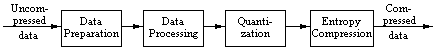
Preparation includes Analog-to-Digital conversion and generating an
approximate representation of the information. In the case of an image, it
is divided into blocks of 8x8 pixels, each pixels represented by a fixed
number of bits.
Processing is the first step of the compression process. If the
domain within which the data is to be compressed needs to be changed, it
can be done at this time. In the case of motion video, a transformation
from the time to the frequency domain may be performed to construct a
motion vector for each 8x8 block in consecutive frames.
Quantization specifies the granularity of the mapping of real numbers
into integers. There is consequently a reduction of space requirements, at the expense of
precision.
Entropy compression is usually the last step. The digital stream
resulting from quantization will be compressed without loss. For example,
Run-length compression replaces a sequence of identical numbers with the
number followed by a special symbol which doesn't occur in the stream
followed by the number of occurrences. E.g., 10000001 would be compressed
to 10!61.
The processing and quantization steps may be performed iteratively several
times in feedback loops. After compression, a data stream is built which
specifies, amongst other things, the compression technique used and any
error correction codes.
Decompression is the inverse of compression. Decompression
techniques can differ from the compression techniques in various ways. For
example, if the applications are symmetric, e.g., dialog applications,
then the coding and decoding should incur more or less the same costs, as
the importance here is the speed factor, rather than quality. However, if
data will be encoded once, but decoded many times, as is the case with an
image or video retrieval system, then whereas the decoding speed must
approximate real-time, the encoding time may be asymmetric to the decoding
time. Usually, better quality/compression ratios are obtained if encoding
time is not a factor.
A data stream is divided into blocks of n bytes, where n > 1, A predefined table contains a set of patterns. For each block, the most similar pattern in the table is identified, and the data stream is gradually replaced with a sequence of pointers to the appropriate pattern index. The decoder, which requires the same table of patterns, generates an approximation to the original data stream. Pattern substitution is also used in text compression. The major difference here is that the decoded data stream must be identical to the original - an approximation may be unintelligible!
This is a variation of run-length coding based on a combination of two data bytes. For a given media type the most common co-occurring pairs of data bytes are identified. These are then replaced in the data stream by single bytes that do not occur anywhere else in the stream.
Different characters do not have to be coded with the same number of bits (e.g., Morse code). Huffman coding analyses the data stream to be compressed, determines the frequency of occurring characters, and assigns shorter codes to frequently occurring characters, and longer codes to those which occur infrequently. For example, given the observed alphabet ABCDE, each character is determined to be a leaf node in a binary tree. Every node in the binary tree will contain the occurrence probability of one of the characters belonging to this subtree. In figure 2 below, the characters A, B, C, D, and E have the following probability of occurrence (based on observation of the data stream):
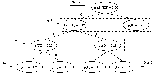
p(A) = 0.16, p(B) = 0.51, p(C) = 0.09, p(D) = 0.13, p(E) = 0.11
(NB: the probabilities are normalized.)
Characters with the lowest probabilities are combined in the first binary
tree (Step 1 in the figure). The next two nodes with the lowest
probabilities are combined into the next binary subtree (step 2). This
process continues until all the remaining nodes have been combined into
subtrees. The allocation of binary 1 and 0 to the paths is arbitrary. The
Huffman table used for encoding a bit stream must be available to the
decoder. Huffman coding is optimal, and guarantees a minimal encoded data
stream. Images are usually represented at the pixel level, and each pixel may be
represented by 8, 16, or 24 bits, depending on the colour-depth. However,
patterns may emerge within the byte representation of pixels. In
order to take advantage of Huffman coding, the pixel representation must
first be transformed into a bit-stream. It is then possible to obtain a
minimal stream length by applying the Hoffman algorithm. The resulting Huffman
table must be available to the decoder to reproduce an image identical to
the original. If the source is a video (a sequence of images), then each
frame may be encoded individually, or else they may be grouped, or the
entire video stream is encoded using the same Huffman table.
Algorithms such as Discrete Cosine Transformation and Fast Fourier Transformation transform the data representation from one mathematical domain (e.g., time) to another which is more suitable for compression (e.g., frequency). The inverse transformation must exist and be known to the decoding process.
Differential encoding is an important feature of techniques used in multimedia systems. In this technique, features of the source data (e.g., an image) are used to calculate the difference between, say, adjacent pixels. For example, neighbouring pixels which together form the background of an image are likely to have identical intensity values. Instead of encoding each pixel value as using 3 bytes, differential encoding would store the value of 1 of the pixels and then difference of the other pixels could be stuffed into individual bits (if their differential value is 0). Run-length encoding can then be performed to further reduce the length of the data stream. In video, this technique could be used to store a frame (known as a key-frame) in its entirety, with subsequent frames being encoded using only the differences from the key-frame. The same techniques can be applied to motion vectors - as an object "moves" across the screen, there will be groups of pixels which differ from frame to frame only by their location in subsequent frames. With audio, subsequent samples are stored only as differences from the previous sample, as it is likely (especially with voice transmissions) that only minor differences will occur in a sequence (Differential Pulse Code Modulation). Audio can be further compressed using silence suppression - data is only encoded if the volume level exceeds a certain threshold.
Date last amended: 2nd September 2002