CSA3020
Lecture 8 - JPEG
References:
Steinmetz, R., and Nahrstedt, K. (1995). Multimedia:
Computing, Communications & Applications. Prentice Hall. Chapter 7.
Steinmetz, R. and Nahrstedt, K.
(2002).Multimedia Fundamentals: Vol. 1. Prentice Hall. Chapter 7,
Section 5.
Aravind, R., et. al., (1993). Image
and Video Coding Standards.
JPEG/JBIG Home page
JPEG
In 1982, Working Group 8 of the International Standards Organization began
working on the standardization of compression and decompression of still
images. In 1986, the Joint Photographers Expert Group (JPEG) was formed,
and in 1992, JPEG became an ISO standard.
The need for image compression is evident in the following example. A
typical digital image has 512x480 pixels. In 24-bit colour (one byte for
each of the red, green and blue components), the image requires 737,280
bytes of storage space. It would take about 1.5 minutes to transmit the
uncompressed image over a 64kb/second link. The JPEG algorithms offer
compression rates of most images at ratios of about 24:1. Effectively,
every 24 bits of data is stuffed into 1 bit, giving a compressed file size
(for the above image dimensions) of 30,720 bytes, and a corresponding
transmission time of 3.8 seconds.
Overview of JPEG
Although JPEG is one algorithm, to satisfy the requirements of a
broad range of still-image compression applications, it has 4 modes of
operation.
Sequential DCT-based
In this mode, 8x8 blocks of the image input are formatted for
compression by scanning the image left to right and top to bottom. A block
consists of 64 samples of one component that make up the image. Each block
of samples is transformed to a block of coefficients by the forward
discrete cosine transform (FDCT). The coefficients are then quantized and
entropy-encoded.
Progressive DCT-based
This method produces a quick low-resolution version of the image, which is
gradually (progressively) refined to higher resolutions. This is
particularly useful if the medium separating the coder and decoder has a
low bandwidth (e.g., a 14.4K modem connection to the Internet, in turn
providing a slow connection to a remote image database). The user can stop
the download at any time. This is similar to the sequential DCT-based
algorithm, but the image is encoded in multiple scans.
Lossless
The decoder renders an exact reproduction of the original digital image.
Hierarchical
The input image is coded as a sequence of increasingly higher resolution
frames. The client application will stop decoding the image when the
appropriate resolution image has been reproduced.
JPEG Operating Parameters and definitions
Parameters
An image to be coded using any JPEG mode may have from 1 to 65,535 lines
and 1 to 65,535 pixels per line. Each pixel may have 1 to 255 components,
although progressive mode supports only 1 to 4 components.
Data interleaving
To reduce the processing delay and/or buffer requirements, up to four
components can be interleaved in a single scan. A data structure called
the minimum-coded unit has been defined to support this
interleaving. An MCU consists of one or more data units, where a data unit
is a component sample for the lossless mode, and an 8x8 block of component
samples for the DCT modes. If a scan consists of one components, then its
MCU is equal to one data unit. For multiple component scans, the MCU
contains the interleaved data units. The maximum number of data units per
MCU is 10.
Marker codes
Different sections of the compressed data stream are delineated using
defined marker codes. All marker codes being with a left-aligned hex "FF"
bytes, making it easy to scan and extract part of the compressed data
without needing to decompress it first.
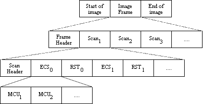
Compressed-image data structure
At the top level of the compressed data hierarchy is the image. A
non-hierarchical mode image consists of a frame surrounded by SOI and EOI
marker codes. A hierarchical coded image will have multiple frames. Within
each frame, a SOF marker identifies the coding mode used. Following an SOF
marker will be a number of parameters and one or more scans. Each scan
beings with a header identifying the components to be contained within the
scan, and more parameters. The scan header is followed by an entropy-coded
segment. The ECS can be broken into chunks of MCUs called restart
intervals, which is useful for identifying select portions of a scan, and
for recovery from limited corruption of the entropy-coded data. Quantization
and entropy-coding tables may either be included in with the compressed
image data, or be held separately.
Sequential DCT
This mode offers excellent compression ratios while maintaining image
quality. A subset of the DCT capabilities has been identified by JPEG for
a "baseline system". This section describes the baseline system.
DCT and quantization
All JPEG DCT-based coders begin by partitioning the image into
non-overlapping 8x8 blocks of component samples. The samples are level
shifted, so that their values range from -128 to +127 (instead of 0 to
255). These data units of 8x8 shifted pixel values are defined by
Sij, where i and j are in the range 0 to 7.
The blocks are then transformed from the spatial domain into the frequency
domain using FDCT:
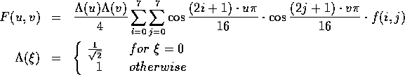
This transformation is carried out 64 times per data unit, resulting in 64
coefficients of Svu.
. The resulting
8x8 matrix will have coefficients ranging from
S00 to
S77, where
S00 is known as the DC-coefficient and
determines the fundamental colour of the data unit of 64 pixels in the
original image. The other coefficients are called AC-coefficients. To
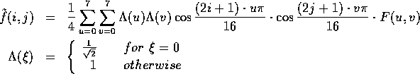
reconstruct the image, the decoder uses the IDCT:
The next step to perform is quantization. The process of quantization
reduces the number of bits needed to encode data and also to increase the
number of zero-valued coefficients. For this purpose, JPEG applications can
specify a table with 64 entries, with a one-to-one mapping between the
values in the table and the DCT-coefficients. Each DCT-coefficient is
divided by its corresponding quantization value, and is rounded to the
nearest integer. JPEG does not specify a quantization table in the
standard. Applications can develop their own tables, which best suit the
type of images used. The quantization table must be available to the
decoder, or else the decoded image may be distorted. Dequantization is
performed by multiplying each DCT-coefficient by the corresponding
quantization value. Notice, however, that in the compression process, the
dividend is rounded - therefore, this technique is lossy, as the
decompression process cannot recover the original values of each pixel!
Most of the areas of a typical image contain large regions composed of the
same colour. After FDCT and quantization, the corresponding S values will have very
low values, although edges in the image will have high frequencies. On
average, images have many AC-coefficients which are almost zero. The image
is further compressed by entropy-encoding the DCT-coefficients in each
data unit.
Entropy Encoding
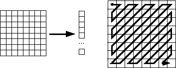
Zig-zag scan.
If a vector of quantized values is constructed using a zig-zag scan shown
in the figure above, then there will usually be a long run of zeros.
First, the zero values of the AC-coefficients are run-length coded.
Then, in the baseline system, the vector is Huffman coded. In
non-baseline systems, Huffman or the more efficient arithmetic coding
can be applied. In both cases, the Huffman or arithmetic tables must be
available to the decoder. This supports sequential encoding, where the
image is encoded and decoded in a single run.
Expanded Lossy DCT-based Mode
In addition to the method described previously, JPEG specifies
progressive encoding. Instead of using just one quantization
step, progressive encoding supports several which are applied iteratively.
Basically, the bigger the quantization block, the less definition is
encoded. So, using an 8x8 quantization table will directly match the
8x8 data blocks extracted from the image in the first place, and apart
from the rounding error, will give a fairly accurate decompressed
image. However, consider the situation where a 64x64 quantization table
is used. Now 8 8x8 blocks will be quantized at a time, resulting in a
significant loss in precision. The greater the quantization table, the
lower the overall precision of the decompressed image. However, if many
quantization tables are used and reapplied to the same
DCT-coefficients, then as the image is being decompressed, it will be
possible to gradually discern more and more definition. The major
advantage is that if the image is being downloaded over a slow network
connection, then the user can see what is in the image faster than if
the sequential encoding has been used. The user can then interrupt the
download if the image is not what s/he was expecting.
Lossless Mode
This mode is used when it is necessary to decode a compressed image
identical to the original. Compression ratios are typically only 2:1.
Rather than grouping the pixels into 8x8 blocks, data units are
equivalent to single pixels. Image processing and quantization use a
predictive technique, rather than a transformation encoding one. For
a pixel X in the image, one of 8 possible predictors is selected (see
table below). The
prediction selected will be the one which gives the best result from
the a priori known values of the pixel's neighbours, A, B, and C.
The number of the predictor as well as the difference of the prediction
to the actual value is passed to the subsequent entropy encoding.
| Selection Value | Prediction |
| 0 | No prediction |
| 1 | X=A |
| 2 | X=B |
| 3 | X=C |
| 4 | X=A+B-C |
| 5 | X=A+(B-C)/2 |
| 6 | X=B+(A-C)/2 |
| 7 | X=(A+B)/2 |
Hierarchical Mode
This mode uses either the lossy DCT-based algorithms or the lossless
compression technique. The main feature of this mode is the encoding of
the image at different resolutions. The prepared image is initially
sampled at a lower resolution (reduced by the factor
2n). Subsequently, the resolution is
reduced by a factor 2n-1 vertically and
horizontally. This compressed image is then subtracted from the
previous result. The process is repeated until the full resolution of
the image is compressed.
Hierarchical encoding requires considerably more storage capacity, but
the compressed image is immediately available at the desired resolution.
Therefore, applications working at lower resolutions do not have to
decode the whole image and then subsequently reduce the resolution.
Back to the index for this course.
In case of any difficulties or for further information e-mail
cstaff@cs.um.edu.mt
Date last amended: 2nd September 2002