A manifold is a space that locally looks like \(n\)-dimensional Euclidean space \(\mathbb{R}^n\).
A 1-D curve locally looks like a line.A 2-D surface locally looks like a plane.
Similarly, a 3-D manifold locally looks like a part of \(\mathbb{R}^3\). If one were able to see it from another dimension, globally, it need not look like Euclidean space \(\mathbb{R}^3\).
Every manifold can be embedded in a Euclidean space of at most twice the dimension, e.g., some curves (the circle) need two dimensions to fit globally, some surfaces need 4, a 3-D manifold may need 5, ...
Orientable Manifolds
The only thing that distinguishes one manifold from another, locally, is the dimension. But they may have different global properties.
Orientability is the property that when a neighborhood of a point wanders far and returns, it is not inverted. All curves are orientable, but not all surfaces are orientable; for those that are, one can distinguish two sides of the surface, as in a sphere (its inner and outer sides).
The Moebius strip is the simplest non-orientable manifold
Connected sum
Click on the curve to connect
Manifolds can be connected together by joining a bridge at local regions. It does not matter where the bridge is made.
The circle joined to any curve does not change it, e.g., two joined loops remain a loop; similarly, any \(n\)-D sphere does not alter a manifold.
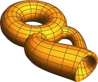
Every manifold can be decomposed into the connected sum of prime manifolds.
1-D Manifolds
The one-dimensional manifolds are the curves. Every curve can be deformed to either a circle or a line.
2-D Manifolds
The two-dimensional manifolds are the surfaces. Every surface can be deformed to one of an infinite number of types:
Surfaces with positive Euler characteristic \(\chi>0\):
Sphere \(\chi=2\)
Flattened 'map' of the sphere.
Projective 'plane' \(\chi = 1\) non-orientable, has only one side.
Surfaces with zero Euler characteristic: \(\chi=0\)
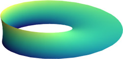
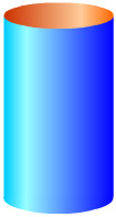
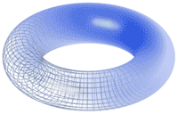
PlaneMoebius strip has one side onlyCylinderTorus
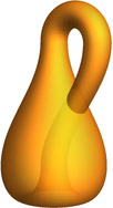
Klein bottle = 2 projective planes joined together; non-orientable — has no inside/outside
Surfaces with negative Euler characteristic: \(\chi<0\)
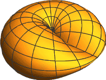
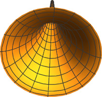
Tractroid part of the larger Hyperbolic plane \(\chi=-1\)
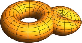
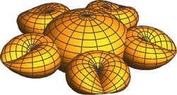
Projective plane + Torus = 3P, three joined projective planes, \(\chi = -1\)
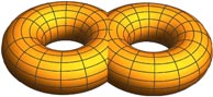
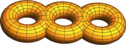
Every compact surface can be deformed into either a number of joined tori or a number of joined projective planes.
\(n\)-Torus = nT \(\chi=2-2n\)\(n\)-Projective = nP \(\chi=2-n\)
Note that adding tori with projective planes gives \(nT+mP = (2n+m)P\).
Connected 3-D manifolds can also be classified, but there are many more types, such as \(\mathbb{S}^3\), \(\mathbb{H}^3\), \(\mathbb{R}^3\), \(\mathbb{S}^2\times\mathbb{R}\), \(\mathbb{H}^2\times\mathbb{R}\), ... But from 4-D onwards they cannot be classified, except the simply-connected ones for 5-D or more.
Differentiation
Because the manifold locally looks like a Euclidean space, its vectors can be 'transferred' to the manifold, forming a tangent space, which could be a line, plane, or \(n\)-D vector space.
A function that is locally linear is called differentiable, \[\color{purple}f(x+h) = f(x) + f'(x)h + \ldots\]
The derivative \(\color{purple}f'(x)\) is a 'matrix' which describes where the tangent vectors in the domain manifold end up in the target manifold.
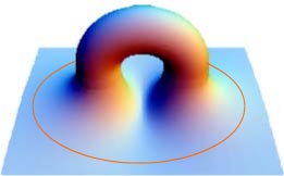
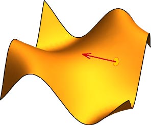
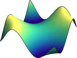
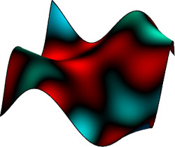
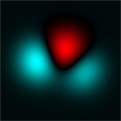
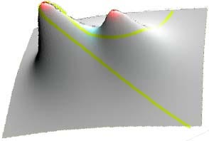
A differentiable real-valued function on a surface. Its derivative or gradient is also denoted \(\color{purple}\mathrm{d}f\).
Locally near any generic point, the differentiable function looks like the inset disk, with values increasing in one direction, except when the derivative is zero.
Critical points are points where a function has zero derivative.
For curves, critical points are of two types, plus higher order degenerate types:
Maximum
Minimum
Degenerate
even type
odd type
On a surface, they are one of the following types:
Maximum
Minimum
Even type
Saddle
Odd type
Higher order
Degenerate types
For a function on any manifold, the number of even critical points minus the number of odd critical points must be equal to the Euler characteristic of the surface (if there are no degenerate points).
\((1+2) - 1 = 2\)
\(1-1=0\)
Vector Fields
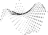
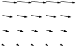
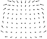
A vector field is a differentiable function which picks a vector at each point on the manifold. Each vector field determines a flow, by following the direction of each vector.
On a surface, a vector field near to a generic point looks like this:
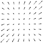
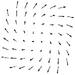
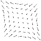
...except at critical points when they look like this (with the even/odd types):
Simple types:
\(+1\) source/sink
\(+1\) vortex
\(-1\) saddle
Degenerate types:
Higher order types:
...
\(+2\) "dipole"
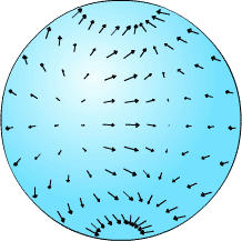
Like scalar fields, the indices of the critical points of any vector field on a manifold, must add up to its Euler characteristic.
3 sources/sinks - saddle = 2
The Euler characteristic for the sphere is 2; so there must be at least one critical point
The Euler characteristic of the circle or torus is 0, so there can be a smooth vector field which is everywhere non-zero.
Derivatives of Vectors
The Lie derivative is a vector field that describes the change of one vector field relative to another:
to see the Lie derivative \(\color{red}{\cal L}_{\color{gray}X}\color{blue}Y\). It drags the vector field \(\color{blue}Y\) along \(\color{gray}X\) and compares the actual vectors with the dragged vectors; the infinitesimal difference is the the Lie derivative.
In one dimension, \(\mathbb{R}\), the derivative becomes the ratio of the infinitesimal change in the output function to the change in the input \(x\), \[\color{purple}\frac{\mathrm{d}f}{\mathrm{d}x}\]
For an orientable manifold there are two ways of taking the usual derivative of a vector field.
the curl \(\color{purple}*\mathrm{d}X\) measures the rate at which a blob flowing along the vector field rotates,
the divergence \(\color{purple}{*\mathrm{d}*}X\) measures the rate at which its volume expands.
Change the vector field. Click at a point in the field to see a blob change at the rates of the div and curl there.
The total of a derivative in a region gives the total of the vector field at the boundary:
Symplectic manifolds have an association between a vector field \(X_H\) and a real function \(H\), such that the function is conserved along a flow on this Hamiltonian vector field. The Lie derivative on the Hamiltonian vector fields takes a special form called the Poisson derivative of the functions, \(\color{purple}\{H,f\}={\cal L}_{X_H}f\).
Geometry
Geometry requires the notion of comparing two entities (vectors, curves, etc.) at two different positions. To do this, there must be a way of transporting or connecting the tangent vectors in the neighborhood, thus allowing a comparison between vectors along a curve. The most common way of doing this is to let transport preserve the lengths of vectors.
Vectors at different points on a curve that have the same direction are called parallel.
A curve whose direction remains "constant" (i.e. parallel) as it moves from point to point is called a geodesic. In Euclidean space they are the straight lines; on the sphere they are the great circles.
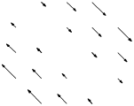
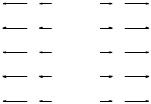
In this example, all the vectors are parallel transported and so are to be considered as the 'same' vectors at different positions. Although the vectors appear distorted and not parallel or of the same length, this is just like the distortion of a world map.
The blue line is a geodesic: it follows the vectors, its tangent remains constant.
Other vectors can twist and stretch when they are carried along: this is due to the intrinsic torsion of the manifold. That is, the parallel transport of vectors in other directions, need not remain parallel to the original.
However, parallel transport depends on the path taken. To the right, a vector is parallel transported in a loop but does not return to the original vector. The extent to which this happens is an indication of intrinsic curvature. In higher dimensions, it may even matter if the loop is knotted or not.
The shortest curve between two not-too-distant points is a geodesic.
Torsion does not affect geodesics, so it is usually neglected when the latter are studied.
Curvature
A one-dimensional curve cannot have intrinsic curvature or torsion. But an \(n\)-D manifold can have a curvature at each point, measured by \(\frac{n^2(n^2-1)}{12}\) numbers, which reduces to just one number \(\color{purple}\kappa\) for surfaces.
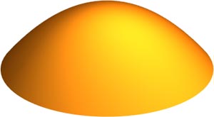
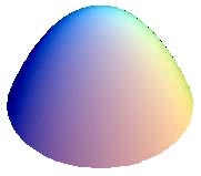
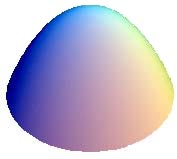
At each point the curvature can be positive, zero, or negative.
\(\kappa\gt 0\)
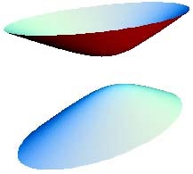
\(\kappa=0\)
'flat'
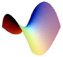
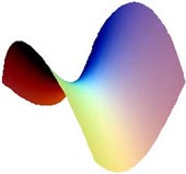
\(\kappa\lt 0\)
The curvature influences the geodesics, focussing them in regions of positive curvature, and dispersing them in regions of negative curvature.
\(\kappa\gt0\)
\(\kappa\lt0\)
The curvature, and geodesics, remain essentially the same when the surface is bent, not deformed.
For any small circle on a surface, \[\color{purple}\begin{align*}\textit{perimeter} &= 2\pi r - \kappa r^3 + \cdots\\\textit{area} &= \pi r^2 - \kappa r^4+\cdots\end{align*}\]
The total curvature around a closed loop equals \[\color{purple}\int\kappa = 2\pi\chi - \text{total exterior angle bend}\] where \(\chi\) is Euler's characteristic of the region in the loop.
In particular,
for the whole surface, \(\int\kappa=2\pi\chi\)
for a polygon of geodesics, \(\int\kappa=2\pi-\text{total exterior angles}\)
There are only finitely many types of compact manifolds whose intrinsic curvature at all points varies between \(\kappa_0\) and \(\kappa_1\).
Isotropic Manifolds
Manifolds that look everywhere the same in all directions are called isotropic. They have constant curvature, so that there are three types: positive, zero, and negative. Locally they look the same, and can be obtained from an \(n\)-D sphere, a flat space \(\mathbb{R}^n\), or a hyperbolic space, respectively.
Planar Geometry, \(\kappa=0\)
The geodesics are called straight lines.
The sum of the exterior angles of a planar polygon is \(2π\) because there is no curvature. In particular, the interior angles of a triangle sum to 180°.
Any two points determine a line; any two lines meet at a point, unless parallel.
Other theorems are mentioned in Vectors.
Surfaces like cones or cylinders really have the same type of local geometry as the plane; they satisfy the same theorems except that geodesics may be closed or self-intersect.
Of course, the whole plane cannot be drawn on the screen. But if we are willing to "bend" reality a bit, it can be fitted inside a disk, by shrinking points towards the origin. Done the right way, straight lines look like "arcs", and "infinity" becomes a circle; parallel lines meet at the same pair of "points at infinity".
Algebraic manifolds are determined by polynomial equations:
Conics
(degree 2 in 2 variables):
Ellipse Lines from focus are reflected to other focus.ParabolaHyperbola
Cubics
(Degree 3 in 2 variables) A sample:
Quadrics
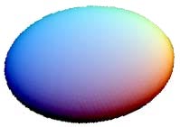
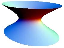
(Degree 2 in 3 variables)
Ellipsoid
Hyperboloid 1
Elliptic Paraboloid
Hyperboloid 2
Cone
Hyperbolic Paraboloid
The intersection of a plane with any quadric gives a conic.
Every embedded surface locally looks like this.
Spherical Geometry, \(\kappa=1\)
Geodesics are great circles. Any two points give a geodesic; any two geodesics intersect.
Similar shapes are congruent.
There are equilateral triangles with any angle between \(60^\circ\) and \(180^\circ\); but there are no rectangles (with all interior angles \(90^\circ\)).
The sum of exterior angles of a spherical polygon equals \(2\pi\) less the total curvature inside, i.e., its area (for a unit sphere). In particular the angles of a triangle sum to between \(180^\circ\) and \(720^\circ\).
Every manifold with varying, but positive, intrinsic curvature must be either compact or a deformed Euclidean space \(\mathbb{R}^n\). Furthermore, when the curvature varies between \(\frac{1}{4}\) and \(1\), the manifold is a deformed sphere \(\mathbb{S}^n\).
Hyperbolic Geometry, \(\kappa=-1\)
Complete negative-curvature surfaces cannot be embedded in \(\mathbb{R}^3\), so to see the hyperbolic plane we need to resort to some visual bending.
A grid of parallel lines, continued from the center, looks like this. Because of the negative curvature, the parallel geodesics diverge from each other. Note that parallelograms (opposite sides parallel) do not have opposite angles equal, and how there can be many non-intersecting lines having different directions.
\[\color{purple}\text{area of triangle }= \pi -(\text{sum of internal angles})\]\[\color{purple}\text{circle: circumference} = 2\pi \sinh(r)\] \[\color{purple}\text{area} = 4\pi\sinh2(r/2).\]
Drag the vertices (slowly) to redraw the triangle.
Drag two vertices to "infinity" to form a geodesic: notice how
there can be several lines going through the 3rd point and not meeting the line;
there are two lines (the other sides of the triangle) that meet it at infinity.
There are equilateral triangles with angles between \(0^\circ\) and \(60^\circ\).
There are no rectangles.
Angles on a chord of a circle are not fixed.
Embeddings
When a manifold is embedded inside another, it acquires a number of normal (perpendicular) vectors. How these change from point to point is measured by the extrinsic curvatures.
Curves embedded in \(\mathbb{R}^3\) have two normals, and two extrinsic curvatures:
the curvature rotates the tangent in the direction of the normal;
the torsion rotates the normal about the curve.
Click to start off a curve, then use W, S to change the curvature, and later A, D to change the torsion.
A constant curvature and torsion produces a helix.
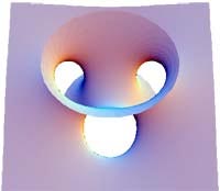
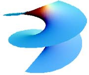
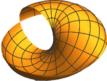
For surfaces embedded in \(\mathbb{R}^3\), there is one normal, with one mean curvature.
Minimal surfaces minimize the area locally: they have zero mean curvature. Such surfaces (soap films) exist over many given boundaries.
In general, for an \(m\)-dimensional manifold embedded in an \(n\)-dimensional ambient space, there are \(n-m\) normals, and hence \(n-m\) extrinsic curvatures.
Complex Manifolds
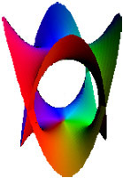
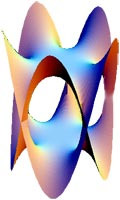
Complex manifolds are manifolds that locally look like the complex numbers \(\mathbb{C}^n\). The most important examples are those that result from polynomial equations:
\(y=x\)\(y^2=x\)\(y^2=x^4-1\) a torus\(y^2=x^5-1\) a 2-torus\(e^y=x\)
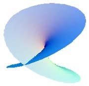
The helicoid minimal surface is an infinitely-twisted plane.
Every differentiable function on a compact complex manifold is constant.
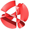
A 4-D K3 manifold: locally looks like the quaternions.
 \(\kappa\gt0\)