Variation of H with T
 

From  one may define c_p, the heat capacity at constant pressure as:

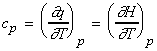………………………………..(eqn. 1)

NOTE: More details on c_v and c_p  may be found here.

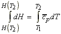
The variation of H with T may hence be studied by solving the differential equation above (i.e. by integration). We shall do this at two levels

(1) Elementary level 
 

Assuming c_p is constant in the temperature region of interest, i.e. for T in (T₁, T₂),.

We may re-write eqn 1. As:
 

i.e.:

i.e.

i.e.:

If T₂ is very different from T₁ than the approximation that c_p is constant in the temperature region of interest cannot be made. Instead we approximate c_p(T) as a polynomial in T, i.e.:

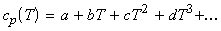
Note: (i) Any function can be expressed as a polynomial; (ii) For most cases, we assume that  gives a well enough description of c_p.

i.e.:

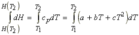
i.e.:

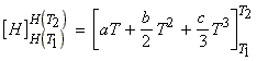
i.e.:

In analogy to eqn. 1, we may write:

…………………… (KIRCHOFF's EQN.)

i.e.:

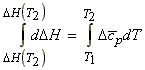
which integrates to:

This may be applied to compute DH_R for reactions at temperature T where T 298K (i.e. not standard). In this case, c_p refers to the reaction, i.e. for the reaction:
 

Example 1:
 

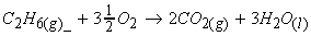
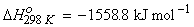
(i)

(ii)

Example 2:
This equation could also be useful, for example, for estimating for T 298K, by letting T₂ = T and T₁ = 298K, i.e.: